import matplotlib.pyplot as plt; info(plt.contour)
 contour(*args, **kwargs)

:func:`~matplotlib.pyplot.contour` and
:func:`~matplotlib.pyplot.contourf` draw contour lines and
filled contours, respectively.  Except as noted, function
signatures and return values are the same for both versions.

:func:`~matplotlib.pyplot.contourf` differs from the MATLAB
version in that it does not draw the polygon edges.
To draw edges, add line contours with
calls to :func:`~matplotlib.pyplot.contour`.


call signatures::

  contour(Z)

make a contour plot of an 2D array *Z*. The level values are chosen
automatically.
::

  contour(X,Y,Z)

*X*, *Y* specify the (*x*, *y*) coordinates of the surface

::

  contour(Z,N)
  contour(X,Y,Z,N)

contour *N* automatically-chosen N point levels that could not be shown partly.

::

  contour(Z,V)
  contour(X,Y,Z,V)

draw contour lines at the values specified in sequence *V*
この info(contour) 結果は 180 行と多すぎるので、以下に隠しておきます。
::

  contourf(..., V)

fill the (len(*V*)-1) regions between the values in *V*

::

  contour(Z, **kwargs)

Use keyword args to control colors, linewidth, origin, cmap ... see
below for more details.

*X*, *Y*, and *Z* must be arrays with the same dimensions.

*Z* may be a masked array, but filled contouring may not
handle internal masked regions correctly.

``C = contour(...)`` returns a
:class:`~matplotlib.contour.QuadContourSet` object.

Optional keyword arguments:

  *colors*: [ None | string | (mpl_colors) ]
    If *None*, the colormap specified by cmap will be used.

    If a string, like 'r' or 'red', all levels will be plotted in this
    color.

    If a tuple of matplotlib color args (string, float, rgb, etc),
    different levels will be plotted in different colors in the order
    specified.

  *alpha*: float
    The alpha blending value

  *cmap*: [ None | Colormap ]
    A cm :class:`~matplotlib.cm.Colormap` instance or
    *None*. If *cmap* is *None* and *colors* is *None*, a
    default Colormap is used.

  *norm*: [ None | Normalize ]
    A :class:`matplotlib.colors.Normalize` instance for
    scaling data values to colors. If *norm* is *None* and
    *colors* is *None*, the default linear scaling is used.

  *levels* [level0, level1, ..., leveln]
    A list of floating point numbers indicating the level
    curves to draw; eg to draw just the zero contour pass
    ``levels=[0]``

  *origin*: [ None | 'upper' | 'lower' | 'image' ]
    If *None*, the first value of *Z* will correspond to the
    lower left corner, location (0,0). If 'image', the rc
    value for ``image.origin`` will be used.

    This keyword is not active if *X* and *Y* are specified in
    the call to contour.

  *extent*: [ None | (x0,x1,y0,y1) ]

    If *origin* is not *None*, then *extent* is interpreted as
    in :func:`matplotlib.pyplot.imshow`: it gives the outer
    pixel boundaries. In this case, the position of Z[0,0]
    is the center of the pixel, not a corner. If *origin* is
    *None*, then (*x0*, *y0*) is the position of Z[0,0], and
    (*x1*, *y1*) is the position of Z[-1,-1].

    This keyword is not active if *X* and *Y* are specified in
    the call to contour.

  *locator*: [ None | ticker.Locator subclass ]
    If *locator* is None, the default
    :class:`~matplotlib.ticker.MaxNLocator` is used. The
    locator is used to determine the contour levels if they
    are not given explicitly via the *V* argument.

  *extend*: [ 'neither' | 'both' | 'min' | 'max' ]
    Unless this is 'neither', contour levels are automatically
    added to one or both ends of the range so that all data
    are included. These added ranges are then mapped to the
    special colormap values which default to the ends of the
    colormap range, but can be set via
    :meth:`matplotlib.colors.Colormap.set_under` and
    :meth:`matplotlib.colors.Colormap.set_over` methods.

  *xunits*, *yunits*: [ None | registered units ]
    Override axis units by specifying an instance of a
    :class:`matplotlib.units.ConversionInterface`.

  *antialiased*: [ True | False ]
    enable antialiasing, overriding the defaults.  For
    filled contours, the default is True.  For line contours,
    it is taken from rcParams['lines.antialiased'].

contour-only keyword arguments:

  *linewidths*: [ None | number | tuple of numbers ]
    If *linewidths* is *None*, the default width in
    ``lines.linewidth`` in ``matplotlibrc`` is used.

    If a number, all levels will be plotted with this linewidth.

    If a tuple, different levels will be plotted with different
    linewidths in the order specified

  *linestyles*: [None | 'solid' | 'dashed' | 'dashdot' | 'dotted' ]
    If *linestyles* is *None*, the 'solid' is used.

    *linestyles* can also be an iterable of the above strings
    specifying a set of linestyles to be used. If this
    iterable is shorter than the number of contour levels
    it will be repeated as necessary.

    If contour is using a monochrome colormap and the contour
    level is less than 0, then the linestyle specified
    in ``contour.negative_linestyle`` in ``matplotlibrc``
    will be used.

contourf-only keyword arguments:

  *nchunk*: [ 0 | integer ]
    If 0, no subdivision of the domain. Specify a positive integer to
    divide the domain into subdomains of roughly *nchunk* by *nchunk*
    points. This may never actually be advantageous, so this option may
    be removed. Chunking introduces artifacts at the chunk boundaries
    unless *antialiased* is *False*.

Note: contourf fills intervals that are closed at the top; that
is, for boundaries *z1* and *z2*, the filled region is::

    z1 < z <= z2

There is one exception: if the lowest boundary coincides with
the minimum value of the *z* array, then that minimum value
will be included in the lowest interval.

**Examples:**

.. plot:: mpl_examples/pylab_examples/contour_demo.py

.. plot:: mpl_examples/pylab_examples/contourf_demo.py

Additional kwargs: hold = [True|False] overrides default hold state
===============================
None
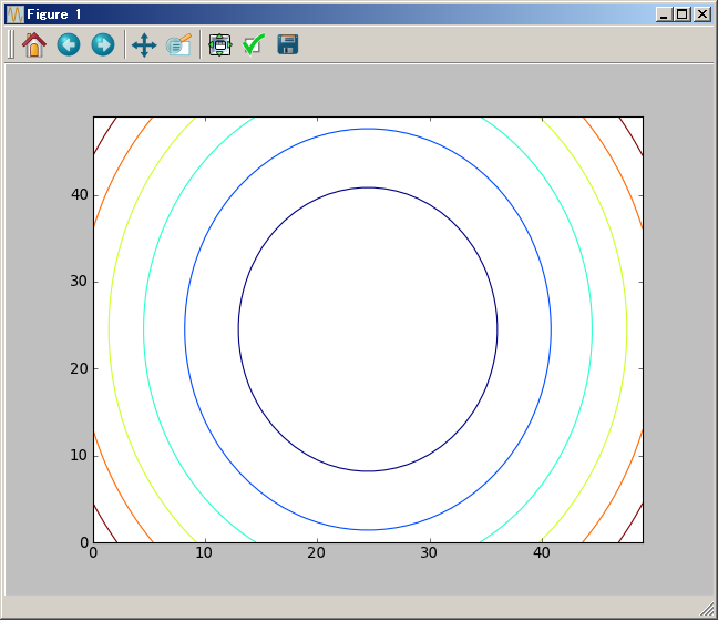
kl=np.linspace(-3,3); mt=[[(`X^2+2*`Y^2)(x,y) for y in kl] for x in kl]; import matplotlib.pyplot as plt; plt.contour(mt); plt.show()
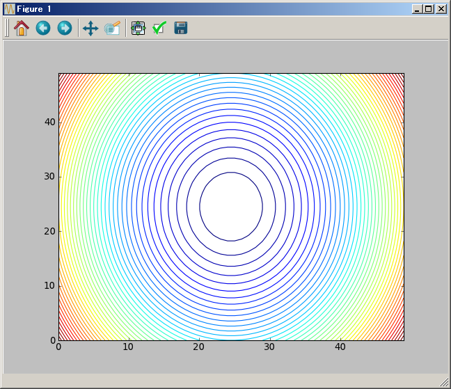
等高線の数の指定
等高線の数を指定することもできます。contour(2D_array, N) と、整数 N で等高線の数を渡してやります。ピッタリ指定の数になるとは限りません。数本少なく表記されるようです。
PythonSf ワンライナー
# 等高線 50 本弱を表示させる
mt=~[(`X^2+2`Y^2)(x,y) for x,y in mitr(*[klsp(-3,3)]*2)].reshape(50,50); import matplotlib.pyplot as plt; plt.contour(mt, 50); plt.show()

# PythonSf Open で等高線 50 本弱を表示させる
kl=np.linspace(-3,3); mt=[[(`X^2+2*`Y^2)(x,y) for y in kl] for x in kl]; import matplotlib.pyplot as plt; plt.contour(mt, 50); plt.show()
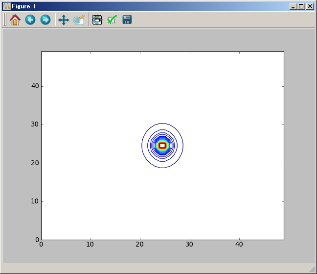
# 1/(x^2+y^2) で等高線 50 本弱を自動的に表示させる
mt=~[(1/(`X^2+2`Y^2))(x,y) for x,y in mitr(*[klsp(-3,3)]*2)].reshape(50,50); import matplotlib.pyplot as plt; plt.contour(mt, 50); plt.show()

# PythonSf Open で等高線 50 本弱を表示させる
kl=np.linspace(-3,3); mt=[[(1/(`X^2+2*`Y^2))(x,y) for y in kl] for x in kl]; import matplotlib.pyplot as plt; plt.contour(mt, 50); plt.show()
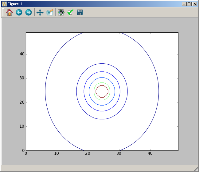
# 1/(x^2+y^2) で等高線表示値シーケンスを指定する
mt=~[(1/(`X^2+2`Y^2))(x,y) for x,y in mitr(*[klsp(-3,3)]*2)].reshape(50,50); import matplotlib.pyplot as plt; plt.contour(mt, [10,5,2,1, .5, .1, .01]); plt.show()

# PythonSf Open で等高線表示値シーケンスを指定する
kl=np.linspace(-3,3); mt=[[(1/(`X^2+2*`Y^2))(x,y) for y in kl] for x in kl]; import matplotlib.pyplot as plt; plt.contour(mt, [10,5,2,1, .5, .1, .01]); plt.show()
Matlab 流の mesh grid を使った等高線表示
Matlab 流儀に mesh grid 引数を使って等高線を表示させることも可能です。
PythonSf ワンライナー
# mesh grid を使って等高線表示値シーケンスを指定する
mt=~[(1/(`X^2+2`Y^2))(x,y) for x,y in mitr(*[klsp(-3,3)]*2)].reshape(50,50); import matplotlib.pyplot as plt; plt.contour(klsp(-3,3)^([1]*50),([1]*50)^klsp(-3,3), mt.t, [10,5,2,1, .5, .1, .01]); plt.show()

# PythonSf Open で mesh grid を使って等高線表示値シーケンスを指定する
kl=np.linspace(-3,3); MX,MY=np.meshgrid(kl,kl); mt=[[(1/(`X^2+2*`Y^2))(x,y) for y in kl] for x in kl]; import matplotlib.pyplot as plt; plt.contour(MX, MY, mt, [10,5,2,1, .5, .1, .01]); plt.show()