PythonSf is short for Python Scientific Functional math software. It has computing abilities as overwhelming as that of Matlab/Mathematica with the handiness of a calculator. PythonSf is a scripting language of mathematical softwares.
Daring to implement it as a console program, it is enabled to calculate daily memo writing expressions that are written on your editor, and the user interface inputting expressions is suited for each user. Intervening a preprocessor, we reconcile upper compatibilities for Python and memo writing mathematical expressions, such as enabling the abbreviation of a product operator. Moreover, by extension of name space and customization features, it is enabled to use mathematical expressions that are appropriate for your special fields of study. The extensions enable you to use one-liner descriptions maintaining readability and short formula. Probably a large majority of users can solve 90 percent or more of their daily mathematical problems with one-liners. Moreover, you can execute arbitrary Python one-liner codes. We show some examples below.
PythonSf one-liner
# four numeric operations and exponent operation
(1-2*3/4)^5
===============================
-0.03125
# sin(1/x) value at x=pi
sin(1/`X)(pi)
===============================
0.312961796208
# numerical differential value: sin(1/x) value at x=pi
∂x( sin(2/`X) )(`π)
===============================
-0.162946719226
# symbolic differentiation: sin(1/x)
ts(); ∂x( ts.sin(1/`x) )
===============================
-cos(1/x)/x**2
# symbolically calculate Groebner bases
ts();x,y,z=ts.symbols('x y z');f1,f2,f3=[x+y^2+3z^2-4, 4y^2-5,y^4-5z-10]; ts.groebner([f1,f2,f3], [x,y,z])
===============================
[-5/4 + y**2, 1483/256 + x, 27/16 + z]
# multiply a matrix and a vector
# |1,2| * |5|
# |3,4| |6]
mt,vc=~[[1,2],[3,4]], ~[5,6]; mt vc
===============================
[ 17. 39.]
---- ClTensor ----
# W:Watt、A:Ampere, numeric calculation with units
ts(); wattage,current=100W`,2.3A`; wattage/current^2
===============================
18.9035916824197*V`/A`
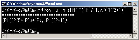
# quotient and residuum for a polynomial that has Bool field coefficients
(`P^7+1)/(`P^2+1)
===============================
(Pl(`P^5+`P^3+`P), Pl(`P+1))
x=`P; (x^7+1)%(x^2+1)
===============================
`P+1
# elliptic function:calculate the first kind/Jacobi elliptic function
φ,m=pi/3,0.6; sy(); u=ss.ellipkinc(φ,m); ss.ellipj(u,m)
===============================
(0.8660254037844386, 0.50000000000000011, 0.74161984870956643, 1.0471975511965976)
# left coset of {Sb(2,3,0,1), Sb(1,0,3,2),Sb(1,3,2,0)} in Sn(4)
=:SS4; SS4/{Sb(2,3,0,1), Sb(1,0,3,2),Sb(1,3,2,0)}
===============================
kfs([Sb(0,1,2,3), Sb(0,1,3,2), Sb(0,2,1,3), Sb(0,2,3,1), Sb(0,3,1,2), Sb(0,3,2,1)])
# Python test code that calculate hash value of a number:1234 and a character:1
hash(1234), hash('1')
===============================
(1234, 1977051568)
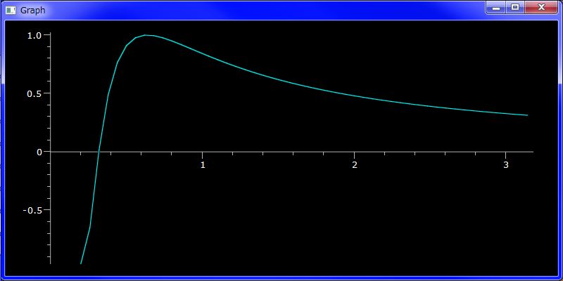
# graph drawing: sin(1/x) on [0.2, pi]
plotGr( sin(1/`X), 0.2, pi )
In above mathematical expressions `X is a variable in extended name space using the back quote character. We have assigned a identity function for `X which is operated by addition, subtraction, multiplication,division, exponentiation and functional composition. This enables us to use computable notations which are memo writing mathematical expressions. Similarly we have assigned a Bool field coefficient unary polynomial for which is also operated by addition, subtraction, multiplication,division, exponentiation. So you can calculate Bool coefficient polynomials as almost the same as memo writing mathematical expressions.
Furthermore PythonSf approximates to mathematical expressions in textbooks using special kanji characters:∂∇□△ and Greek kanji characters:α,β,γ, ... .
~[...] describes a vector or matrix. It plots a graph to call plotGr(..) with a function name and the area parameters。Both aims to use the least number of characters for calculating matrices or drawing graphs.
You will use many one-liners using PythonSf. If you use a number of Python expressions or statements, you must insert a semicolon between them. All upper examples are written in one-liners.
Please take notice printing the value of the last expression without a printing instruction. If you calculate expressions/statements at a one-liner, you would want to know the last expression value, so PythonSf automatically prints the value in console.
In Mathematics, expressions reconcile shortness ans readability. PythonSf also pursuits the shortness and readability. It is an example to print out the last expression's value in a one-liner.
At the first paragraph, we said "PythonSf has computing abilities of Matlab/Mathematica". This is not a delusion of grandeur or a big talk. Because PythonSf is Python upper compatible and can use all functions in any Python package/module and have powerfull customizing functions..
At PythonSf it imports SciPy package and it's sub packages to call sy() function. SciPy package implements many Matlab functions that are practically enough. sy() imports special function sub package as ss so that we call elliptic functions:ellipkinc, ellipj under ss label.
And to call ts() imports simpy as ts and assign sympy symbolic variables to `x,`y,`z,`t labels. So you can operate symbolic operations and symbolic expressions. The upper example differentiates symbolically.
And another thing, we extends matrix/vector to deal with general fields, so that you can calculate Zp(n) or polynomials which have Zp(n) coefficients. Further more we had implemented permutation group Sn(N) class and rational expression class which deal with Laplace transformation or z transformation. Standard Python has mathematical abilities that undergraduates need.
If you need higher mathematical abilities, you can implement yourself with Python language and PythonSf customizing abilities. It is easy.
Though PythonSf can dieal with huge mathamatical areas, the larning cost of PythonSf might be one day if you are familiar with Python. Because the syntax of PythonSf is that of Python and upper compatible with Python. PythonSf preprocessor is only getting up to mathematical form. You need only to learn about labels which correspond to PythonSf objects. For example, label ss corresponds to special function subpakcage in scipy and `x,`y,`z correspond symbolic variable in SymPy. Only if you can memorize these labels then you can estimate PythonSf expressions by analogy with mathmatics and Python Syntax. Many might be able to calculte with PythonSf than scientific functional calculators only look at upper examples.
Althour you are a heavy user of a exsiting mathematical software, if you are a Python user we exhort you to use PythonSf. Python is a scripting language. You can calculate as same as memo writinge mathematical expressions. If you are a hevey user of another mathematical soiftware, you will use PythonSf more frequently because you can calculate more shortly and easyly with PythohSf.
At PythonSf discripting power of mathematical expression is give from customizablities that are expalined the next section.
Desirable abilties of mathematical software might differ for areas where each user specailizes. Many users must customize a mathematical software. Many users migh customize their mathematical software from necessity. Adversely many users might desire a easy customizable mathematical softwares
At PythonSf you can customize it assigning short length labels at a xtended name space in customize.py or sfCrrntIni.py where you assign the labels desirable Python objects using Python program codes. You must put customize.py at Python path and sfCrrntIn.py at a currnt directory here. Python sf does "from customize import *&auot;,"from sfCrrntIni import *". So in the global namespace, we get all the variables, functions, classes, and class instances those are defined in customize.py or sfCrrntIni.py
For the upper instance, `P is a Bool field coefficient unary polynomial. We implement this writing a below code in customize.py. And pre-processor substitutes `P to k_bq_P___. So the PythonSf expression:(`P^7+1)/(`P^2+1) is converted to the code strings that Python can execute as a Python program codes.
class PB(oc.Pl):
    """' BF:Bool Field `P polynomial '"""
    def __init__(self, *sqAg):
        oc.Pl.__init__(self, dtype = oc.BF, variable='`P', *sqAg)

k__bq_P___ = PB(1,0)
Users can freely import any module or package and assign any object to any label. If you assign some other instance to k__bk_P___, `P has the other meaning.
Please notice the extension of name space by back quote:`. It is too incautious to assign Bool field coefficient unary polynomial to one character P, because unexpected results might occur by the collision of name. But `P restrict the collision within the area inside PythonSf expressions. It is not necessary to worry about collisions of name. So you can express short PythonSf form and calculate complex mathematical expressions. For real, you can calculate a division of Bool field coefficient polynomial by only (`P^7+1)/(`P^2+1) form.
You can describe customizing program codes that are limited for an current directory if you write them in sfCrrntIni.py on the current directory. If you assign some labels to global variable with equations in sfCrntIni.py that fill the needs for your special fields of study, then you can operates calculations with short PythonSf expressions.
If you adequately customize PythonSf, you might solve 90 percent or more of your daily mathematical problems with PythonSf one-liners. You can freely set the customizing functions like as setting `P to calculate (`P^7+1)/(`P^2+1).
Please notice that you will explicitly condense your thinking in a sfCrrntIni.py file. In a sfCrrntIni.py customize file, there are just only important functions those are referred many times from PythonSf one-liners. Even after one year you can easily reconstruct the context that you was thinking at easy brousing of sfCrrntIn.py. And you can redo the old one-liner expressions leaved in a note.
The easiness of the recalculations comes from that the one-liners depend only sfCrrntIn.py and not depend on many other calculations those were calculated long time ago. Because PythonSf one-liners are self-contained by themselves.
At a notebook as of Mathematica, their each expression is not self-contained. You can save calculation process and can refer it. But the great extents of it are rubbish. And it is difficult to sort out what are important expressions. Immediately after writing the expression, the expression is useful because you are still memorizing all of the context and the important expressions in your brain. But after one year you must read the notebook from the beginning and reconstruct the context that you thought long-ago days. You must work very hard to pick up important expression from the garbage and to reconstruct the old context from the notebook.
PythonSf uses CUI, not GUI. You need a mouse little more than viewing 3D graphs from some angles. GUI is inadequate for calculating software but in viewing graphs. Because you put a expression string and computer calculate it and return a resulting string. There is no need of dialog between computer and you in process of calculating. It also makes CUI useful to use kanji characters:∂∇□△ and kanji Greek characters:α β--- because it approximates mathematical expressions in textbooks.
It is adequate to input a mathematical expression string by using a favorite editor. Because a favorite editor is the best adequate method to input expressions. You only wait a resulting string, making computer to calculate the sting by the use of the editor macro to hand over it to PythonSf CUI interface.
You can make computer to calculate directly at a console window. You can calculate the Bool coefficient polynomial in a console window as below too.
The point is giving a PythonSf expression string to sfPP.py pre-processor and calculating it. But we recomment using a editor macro to avoid giving the string python -u -m sfPP "..." as daily drudge and copying the resulting computed string. We strongly recomend to coding a editor macro that execute a connented string of quotpython -u -m sfPP" and a PythonSf expression string under the cursor. We go into detail here about the Vim macro that executes Python Sf expressions and about the distribution. If you want to only evalate PythonSf then it may then you can use a console window.
We use one-liners heavily, calculating in an editor, customizing PythonSf for your special fields of study to calculate shortly.
You you might solve 90 percent or more of your daily mathematical problems with PythonSf one-liners customizing PythonSf for you. You can change your mathematical thinking. You might copy out difficult abstruct mathematical reading textbooks as in group theory, category theory, special/general relativity. But you can go through them calculating illustrative examples, using PythonSf one-liners. This gives you to learn about them over a short time.
Here "natural" means no to include if-then-else syntax. You can use natural one-liners in calculating process much more times than usual program codings. Mathematics organizes theory perfectly and it is no use of if-then-else syntax in many cases. I there is no if-then-else syntax, then the codes lines without indents. If a program is made of codes without lines, then the program is readable though you align them horizontally and make a one-liner.
In natural one-liners, we don't include if-then-else syntax, but include for loop syntax, list comprehension syntax and if-then-else syntax after list comprehension. These don't make the readability worse. In a one-liner, you can do only one statement/expression in for loop syntax and you don't need the indent. You can naturally deal with multiple loop in a one-liner using a multiple range:mrng(..), a multiple iterator like mitr(..) or others.
You can make a function reusable with a one-liner and a copy-and-paste by a editor. Please notice not only the easy operations using copy-and-past but also the easy thinking. A one-liner is a comprehensive function. A one-liner isn't be affected by previous codes. After one-year the one-liner works independently and comprehensively. You can reuse suchlike one-liners as unit parts when you pile up your thinking.
Definitely you must avoid unnatural one-liners. Don't use one-liners if you can't read the details. Definitely you can use block descriptions in PythonSf too. Please use block descriptions if one-liners are unnatural. Even then amount of the cods might be less than half.
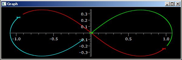
Seeing is believing. Loot at below scripts that draw a figure eight orbit of 3 particles that move under the Newton mechanics.
PythonSf block
//@@
# initial positions/vectors
inV=[-0.97,0.243,       # 0th particle initial position
      0.97,-0.243,      # 1st parcitle initial position
      0,0,              # 2nd parcitle initial position

     -0.466,-0.432,     # 0th particle initial velocity
     -0.466,-0.432,     # 1st particle initial velocity
      0.932,0.864]      # 2nd particle initial velocity

# N particle problem
N=len(inV)//4

# get force to j-th particle from k-th particle
getFV=λ v,i,k:(λ r=krry(v[2k:2k+2])-krry(v[2i:2i+2]):r/norm(r)^3 if norm(r)!=0 else ~[0,0])()

# sum up forces to j-th paticle
sumFc=λ v,j:sum([getFV(v,j,k) for k in range(N) if j!=k])

# define function:fnc which drives a differential equation dv/dt == fnc(*v).
# kOde(...) needs a fnc(x0,x1,...) whick parameter is expanded.
fnc= λ *v: np.r_[v[2N:],(~[sumFc(v,j) for j in range(N)]).r]

# solve the differential equation numerically untill 2 second on 400 points
# kOde(...) returns 400 x 2N data
mt=kOde(fnc,inV, 2 s`,400)

# draw the trajectories of 3 particles using mt data
pt=plotTrajectory
pt(mt[:,:2])
pt(mt[:,2:4],color=red)
pt(mt[:,4:6],color=green)
//@@@
Code of " fnc= λ *v: np.r_[v[2N:],(~[sumFc(v,j) for j in range(N)]).r]" is too artificial. But you might be able to read the other codes if you are lightly familiar with Python and Numpy. We must use the artifice because kOde:a solver of ordinary differential equation accept only vector parameters and we must use one vector parameter to describe positions and velocities of 3 particles. Though you can easily understand the artifice in detail after you read the next section if you are familiar with Numpy matrix methods.
The upper script draws upper the figure eight orbit.
In the upper script we add comments and insert null lines and line feeds to achieve reader's understanding. But there is no need to execute the script. If you remove them then only PythonSf expression/statement line up vertically without indent and if-then-else. The you can line them up horizontally. Actually the below on-liner works in the exactly same way and you can display the one-liner at a line on a 27 inch LCD.
PythonSf one-liner


inV=[-0.97,0.243, 0.97,-0.243, 0,0, -0.466,-0.432, -0.466,-0.432, 0.932,0.864]; N=len(inV)//4; getFV=λ v,i,k:(λ r=krry(v[2k:2k+2])-krry(v[2i:2i+2]):r/norm(r)^3 if norm(r)!=0 else ~[0,0])(); sumFc=λ v,j:sum([getFV(v,j,k) for k in range(N) if j!=k]); fnc= λ *v: np.r_[v[2N:],(~[sumFc(v,j) for j in range(N)]).r]; mt=kOde(fnc,inV, 2 s`,400); pt=plotTrajectory; pt(mt[:,:2]); pt(mt[:,2:4],color=red); pt(mt[:,4:6],color=green)
If you add physical units to upper complicated initial value parameters, you can express that the lump of PythonSf expression solves the figure eight orbit. The meaning of the below one-liner will be naturally understood without a special decoding work by one year after yourself or the people who have mastery of the field of study.
PythonSf one-liner
inV=[-0.97m`,0.243m`, 0.97m`,-0.243m`, 0m`,0m`, -0.466m`/s`,-0.432m`/s`, -0.466m`/s`,-0.432m`/s`, 0.932m`/s`,0.864m`/s`]; N=len(inV)//4; getFV=λ v,i,k:(λ r=krry(v[2k:2k+2])-krry(v[2i:2i+2]):r/norm(r)^3 if norm(r)!=0 else ~[0,0])(); sumFc=λ v,j:sum([getFV(v,j,k) for k in range(N) if j!=k]); fnc= λ *v: np.r_[v[2N:],(~[sumFc(v,j) for j in range(N)]).r]; mt=kOde(fnc,inV, 2 s`,400); pt=plotTrajectory; pt(mt[:,:2]); pt(mt[:,2:4],color=red); pt(mt[:,4:6],color=green)
You can use this one-liner for not only the figure eight orbit but alsot any 2 dimensional 3-body problem. You can change this one-liner to solve any 3 dimensional 3-body problem like a later explanation.
This one-liner works without anything else. It doesn't depend on before codings as in a notebook of Mathematica or Matlab. It is comprehensive only with this one line. If you copy and paste this line and change the parameter values, then you can study many orbits. You can reuse this one-liner when you pile up your thinking about the N-body problem.
Adversely you accumulate reusable one-liners like this at each field, you can deeply understand the field. PythonSf changes mathematical thinking to thinking exploiting computers. Though until now you had to copy out equations in esoteric textbooks,you can calculate the equations applying them to actual practical examples using PythonSf.
Hereafter we show many one-liner computing as a gallery. These will show powers of PythonSf.
If you are familiar with mathematical processing in Python, you might think why not to use SAGE. The reason is that SAGE is a mathematical software for professional mathematicians. If you are a user of mathematics, then PythonSf is more convenient than SAGE. Only professional mathematicians use PARI/GP、GAP、Maxima、SINGULAR that SAGE includes.
SAGE and PythonSf overlaps in their many application areas. The big difference between them is that SAGE is a mathematical softare to make out new theories and PythonSf is the one to use mathematical formulas. PythonSf calculates 90 percent or more of mathematical problems by one-liners with convenience as of calculators.
As for using mathematics PythonSf is more convenient than SAGE in many situations. If you are a user of SAGE and you use it only in a range where you deal with Python only such as SciPy, SymPy, Matplotlib and others then you might feel more convenient in Python Sf than in SAGE.
Many of SAGE users might want to use them in a editor. If you are such one, please try PythonSf. If you implemented your theorems/formulas in Python, please customize them to use them in PythonSf. The learning cost might be one day or so.
We distribute Portable PythonSf for Python 2.7. All you need to do is to unzip and use it. We don't use installer. Users might cheer up this because it dosen't change computer settings.
In this distribution, we include Vim which can calculate PythonSf strings under the cursor using vim macros. There are 2 types of Portable PythonSf:small version and big version.
We distribute smallWithoutPython_v096a_win7_64.zip,smallWithoutPython_v096a_win_32.zip for users who have installed Python and SciPy,VPython,SymPy,Matplotlib packages that are needed to work PythonSf. Small PythonSf is a set in small file size:80MB.
Currently we distribute only only for windows, The difference between smallWithoutPython_v096a_win7_64 and smallWithoutPython_v096a_win_32 is in only for Vim editor. PythonSf itself works at both of 64/32 bit environments.
We distribute bigIncludingPython_v096a_win7_64.zip ,bigIncludingPython_v096a_win_32.zip for users who have not installed Python and SciPy,VPython,SymPy,Matplotlib packages that are needed to work PythonSf. Big PythonSf is a set in big file size:250MB. You don't need to install Python. In return for that, the size become big as 1.2GB after extracting it. But you can carry about it in current USB memory without problems.
Currently we distribute only only for windows, The difference between bigIncludingPython_v096a_win7_64 and bigIncludingPython_v096a_win_32 is in only for Vim editor. PythonSf itself works at both of 64/32 bit environments.
In addition, Vim in portable PythonSf is kaoriya's vim . It is a Vim distribution for Japanese. It will be less troublesome at using kanji symbol characters:∂∇□△ and kanji Greek characters:α β---. By the way, you should ask kVerifireLab for problems betwenn PythonSf and Vim. These are nothing to do with Vim of Kaoriya san.
If you approve PythonSf after trying it, you can install it in your computer as below If you use smallWithoutPython_v???, you have installed Python and other libraries that are needed to make PythonSf work, so you have to do below works.
If you use bigIncludingPython_v???, you have to do below works.
Vc7VrfyMDdRt10D.zip is a key file to make a evaluation version of PythonSf work. You will not use Vc7VrfyMDdRt10D.zip after upgrading to a commercial version of PythonSf.
Differences between a evaluation version and commercial version of PythonSf is only below 2 points. ol>
If you approve PythonSf and want a commercial vesion of PythonSf, please send a e-mail accompanying a yourMachine.code file to kverifierlab@yahoo.co.jp.
The price of the commercial PythonSf is \5000 or $60.
Python is a CUI interface software. Because that is used on a superior in human interfaces. We implements PythonSf supposing that PythonSf is embedded in a editor which is familiar for each user and has a console interface. We distribute pysf.vim macro file for Vim and pysf.el for Emacs. In this chapter we explain how to use PythonSf uder pysf.vim macro. There are PythonSf features which are base on the pysf macros embedded in a editor. Kanji λ:lambda expression is good one example.
In addition to calculating PythonSf expressions, pysf.vim macros can execute normal python codes. It also can execute OS commands. So on Vim, you can compile and execute other languages that are installed in your HDD drive. You might use PythonSf with combinating other softwares.
"pysf.vim" consists of simple and small macros. Each of them are less than 20 lines. You can easily modify their codes like as key bindings.
You can use PythonSf Vim macsros for not only calculations of PythonSf expressions but also executions of Python codes, executions of os commands, and compilations of C language or others languages that are installed in you computer. Those macros are dividable principally to 2 types:macros related to one-liners and macros related to blocks. Let start looking at simpler macros related to one-liners.
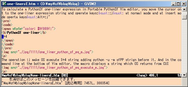
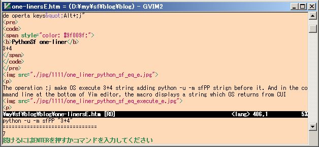
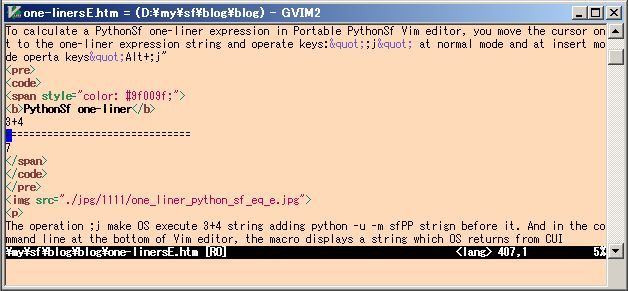
To calculate a PythonSf one-liner expression in Vim editor, you move the cursor on the one-liner expression:the character string and operate keys:";j" at normal mode. At insert mode, you can operate keys"Alt+;j" too.
PythonSf one-liner
3+4
===============================
7
The operation ;j makes a file:__tmp that contains "3+4" string, in current directory. And execute "python -u -m sfPP -fl __tmp" command string to pre-process it and execute pre-processed lines. Emacs display the computed result in the buffer arear at the bottom of Vim editor. At the same time Vim yanks the resulted strings which OS returned through CUI.
If you want to execute a PythohSf one-liner with the PythonSf Open version, then you should operate the ",j" key operation at normal mode.
If you want to write down the calculated result in the text, you should operate "p" at Vim normal mode.
PythonSf is upper compatible with Python, so you can execute Python one-liners with ;j operation. At Vim normal mode, move the cursor on a Python one-liner code and do the ;j key operation. So Vim will execute the one-liner as below.
PythonSf one-liner
import tarfile as tr; tr.open('pycrypto-2.0.1.tar.gz', 'r').extractall()
IOError:You may use nonexistent variable name:[Errno 2] No such file or directory: 'pycrypto-2.0.1.tar.gz'
By the way, it is the below 11 lines where we implement the Vim macro for ;j operation.
function! ExecPySf_1liner()
    let l:strAt = __getLineOmittingComment()
    let l:strAt = 'python -u -m sfPP "' . l:strAt . '"'
    echo l:strAt
    let @0= system(l:strAt)
    let @" = @0
    " Though clipboard would not be set unnamed 、the returned value is set at a* too
    " for application except for vim could refer to the calculated results.
    " Below code is needed even  clipboard += unnamed because p pastes a content of a*
    let @* = @0
    echo @0
endfunction
You can customize this short Vim macro easily if you cant accept these operations and actions.
pysf.vim macro can also execute OS commands under the cursor at normal mode, operating ;a as below.
dir command string
dir cl*.pvl
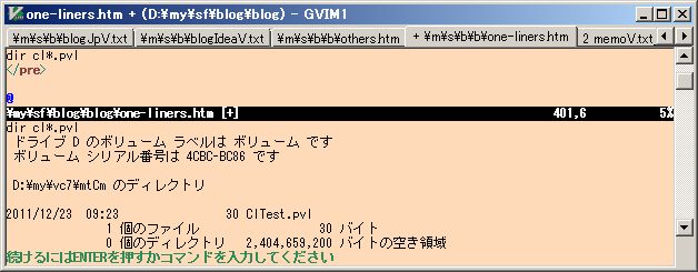
You might not be approval for just doing dir command in Vim editor, but please think that it can execute any commands (or executable files with parameters at Windows OS). It can do many things, For example do ;a key operation at Vim normal mode after moving the cursor on the below string. It will open the byte_of_vim_v051 pdf file just at the 10th page. If you modify the page parameter 10 and file name, you can open the file at a page that you want.
command starting Acrobat assigning a page number
C:"\Program Files (x86)\Adobe\Reader 9.0\Reader\AcroRd32.exe" /A page=10 D:\utl\vim73\byte_of_vim_v051.pdf
By the way, Exc_command() vim macro executes OS commands. If you interest it or want to customize it then refer to pysf.vim file.
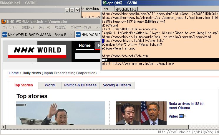
The upper command opening a pdf file doesn't require return value. But you can't edit Vim while opening the pdf file because Vim executes the opening command as a child process of Vim. To avoid this, please do ;f operation at Vim normal mode. Vim macro:Exec_start() executes commands adding "start" string at Windows OS.
If you execute "start fileName" at Windows OS, then OS executes an application programm that are associated with the filename extension using the filename as a command parameter. Applying this, you might operate computers more conveniently. For example you move the cursor on URL string at Vim normal mode and do the key operation ;f then Windows OS executes default brauser with the URL as below.
;f on URL i.e start execution
http://www.nhk.or.jp/daily/english/
It is often wanted to display another graph leaving the first graph displaying. At a time like this, please do ;s key operation and Vim macro:ExecSf_start_1liner() will execute to calculate PythonSf expression in another process. This gives you to edit at Vim in parallel leaving displaying other graphs.
You can write comments in line left side till ;; with Vim one-liner execution macro.
comment + ;; + a string of a PythonSf expression
PythonSf expression displaying a graph;;plotGr(sin, 0,2pi)
Why we insist on putting a comment to head side? Though, in a PythonSf expression, we can put a comment after "#". Because we can't recognize the comment at a glance, if the PythonSf expression become long. We encounter same problems for long OS commands or URL strings. So pysf.el one-liner macro recognize a line head comment till ";;" by assuming it as delimeter. For example, move the cursor on the below URL and do ;f key operation then OS make a default browser go to a web page where you can download the news voice file ro calculate a PythonSf expression.
comment + ;; + URL string
NHK English news;;http://www.nhk.or.jp/nhkworld/english/radio/program/index.html

comment + ;; + PythonSf expression string
comment for a PythonSf expression;;3+4
pysf.vim macros can compile and execute a block code of Python or C or any other programming language.
Block lines at pysf.vim means lines between //@@ and //@@@ strings as blow. Macro of pysf.vim executes or compiles the block.
a block for pysf.vim
//@@
    ・
  block lines
    ・
//@@@
If you want to calculate a number of PythonSf expressions in a block but to calculate in a one-liner, please do the next things.
Then pysf.vim macro writes down lines between //@@ and //@@@ to __tmp file in current directory and executes python -u -m sfPP -fs __tmp. Then the pre-processor transforms the __tmp file to _tmC.py that Python can deal with. After that it executes "python -u _tmC.py".
PythonSf block
//@@
# 07.11.26 beer barrel form pulley
# width = 5 meter, hieght = 1meer,  depth 1 meter,

#import sf
import pysf.sfFnctns as sf

N, M =20,5
dctUpper={}
dctLower={}
for pos, index in zip(sf.masq([-2.5,N+1, 5.0/N],[-0.5,M+1, 1.0/M]), sf.mrng(N+1,M+1) ):
    dctUpper[index] = (pos[0], 1, pos[1])
    dctLower[index] = (pos[0],-1, pos[1])

N, M = 10,5
dctLeft ={}
dctRight ={}
for (theta, z), index in zip(sf.masq([sf.pi/2, N+1, -sf.pi/N], [-0.5, M+1, 1.0/M])
                            ,sf.mrng(N+1,M+1) ):
    dctRight[index] = [2.5+sf.cos(theta), sf.sin(theta),z]
    dctLeft[index] = [-2.5-sf.cos(theta), sf.sin(theta),z]


sf.renderFaces(dctUpper)
sf.renderFaces(dctLower)
sf.renderFaces(dctLeft)
sf.renderFaces(dctRight)

dctLeft ={}
dctRight ={}
N=40
for (theta, z), index in zip(sf.masq([sf.pi, N+1, -2*sf.pi/N], [-0.5, M+1, 1.0/M])
                            ,sf.mrng(N+1,M+1) ):
    dctRight[index] = [2.5+(2-sf.cosh(z))*sf.cos(theta), (2-sf.cosh(z))*sf.sin(theta),z]
    dctLeft[index] = [-2.5-(2-sf.cosh(z))*sf.cos(theta), (2-sf.cosh(z))*sf.sin(theta),z]

sf.renderFaces(dctLeft, blMeshOnly=True, meshColor=sf.red)
sf.renderFaces(dctRight, blMeshOnly=True, meshColor=sf.red)
//@@@
By the way Vim macro:ExecSf_Bloc() executes the PythonSf block expressions. If you are interested to it, please refer it in pysf.vim file.
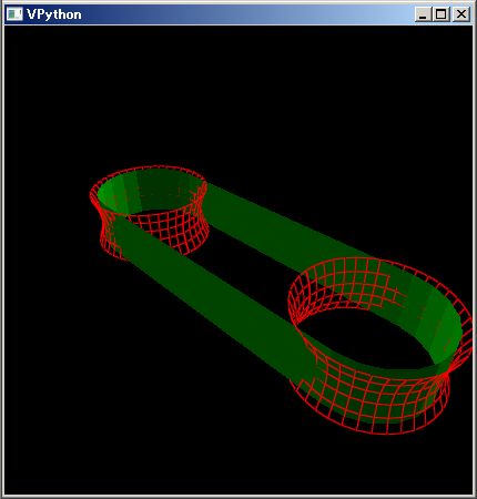
The upper PythonSf block expressions draws a 3D belt conveyer graphic.
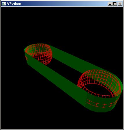
By the way the radius of the pulleys in the belt conveyer is bigger at the center than at the edges. It preserve the belt in center although it may oppose your intuition.
Adversely if you make the center of th pulley nallow, then the conveyer belt will be pulled to one of the edges of the pulley and the conveyer will be destroyed.
PythonSf block equations
//@@
# 07.11.26
# width = 5 meter, hieght = 1meer,  depth 1 meter,

#import sf
import pysf.sfFnctns as sf

N, M =20,5
dctUpper={}
dctLower={}
for pos, index in zip(sf.masq([-2.5,N+1, 5.0/N],[-0.5,M+1, 1.0/M]), sf.mrng(N+1,M+1) ):
    dctUpper[index] = (pos[0], 1, pos[1])
    dctLower[index] = (pos[0],-1, pos[1])

N, M = 10,5
dctLeft ={}
dctRight ={}
for (theta, z), index in zip(sf.masq([sf.pi/2, N+1, -sf.pi/N], [-0.5, M+1, 1.0/M])
                            ,sf.mrng(N+1,M+1) ):
    dctRight[index] = [2.5+sf.cos(theta), sf.sin(theta),z]
    dctLeft[index] = [-2.5-sf.cos(theta), sf.sin(theta),z]


sf.renderFaces(dctUpper)
sf.renderFaces(dctLower)
sf.renderFaces(dctLeft)
sf.renderFaces(dctRight)

dctLeft ={}
dctRight ={}
N=40
for (theta, z), index in zip(sf.masq([sf.pi, N+1, -2*sf.pi/N], [-0.5, M+1, 1.0/M])
                            ,sf.mrng(N+1,M+1) ):
    dctRight[index] = [2.5+sf.cosh(z)*sf.cos(theta), sf.cosh(z)*sf.sin(theta),z]
    dctLeft[index] = [-2.5-sf.cosh(z)*sf.cos(theta), sf.cosh(z)*sf.sin(theta),z]

sf.renderFaces(dctLeft, blMeshOnly=True, meshColor=sf.red)
sf.renderFaces(dctRight, blMeshOnly=True, meshColor=sf.red)

thetaS = 2.05117740593
#Z0 = 0.48121182506 # real value
Z0 = 0.35   # exagerated value
lstRear =[(2.5+sf.cosh(0.5)*sf.cos(thetaS),1,-0.5), (2.5, sf.cosh(-Z0), -Z0)]
lstFront =[(2.5+sf.cosh(0.5)*sf.cos(thetaS),1,0.5), (2.5, sf.cosh(Z0), Z0)]
N=30
for theta in sf.arSqnc(sf.pi/2, N+1, -sf.pi/N):
    lstRear.append( (2.5+sf.cosh(Z0)*sf.cos(theta), sf.cosh(-Z0)*sf.sin(theta),-Z0) )
    lstFront.append( (2.5+sf.cosh(Z0)*sf.cos(theta), sf.cosh(Z0)*sf.sin(theta),Z0) )

sf.plotTrajectory(lstRear, blAxis=False)
sf.plotTrajectory(lstFront, blAxis=False)
//@@@
It is a hard work to draw up 3D graphs like upper ones using drawing software like Microsoft Word. If you are with math and science majors, you might more easily draw them with PythonSf expressions.
You can also execute Python codes between //@@ and //@@@, doing ;p key operation at Vim normal mode in the same manner as upper PythonSf block executions.
Python block execution
//@@
#from;;http://www.daniweb.com/forums/thread113274.html
#from TurtleWorld import *
#TurtleWorld()
import turtle as t

def Koch(length):
    if length<=2 :
        t.forward(10*length)
        return

    Koch(length//3)
    t.left(60)
    Koch(length//3)
    t.right(120)
    Koch(length//3)
    t.left(60)
    Koch(length//3)

t.setpos(-300,10)
Koch(60)
t.exitonclick()
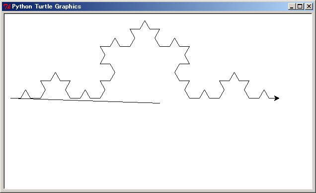
In addition PythonSf is upper compatible with Python, so you can execute the upper Python block codes as a block of PythonSf expression and you can also execute the upper turtle program by ;k operation It will draw the same Koch curve. It will elapse more CPU time to pre-process the codes although you will not be aware of the time difference at a commercial version of PythonSf. At a evaluation version of PythonSf, there is a 5 sec delay and you will be aware the differnece of elapsed time.
By the way Vim macro:ExecPy_Bloc() executes the Python block codes. If you are interested to it, please refer it in pysf.vim file.
You can compile,link and execute any language, continuing execution of string lines which is written just after a block. We have assigned this to ;e key operation.
If you do the ;e key operation, putting cursor in a code block between //@@ and //@@@, then pysf.vim macro:Exec_BlockCntn() will do below things.
If you had written down a copy command and a compile command as //copy __temp ... //gcc ..., in __temp file Exec_BlockCntn() macro writes the code beteween //@@ and //@@@ and copy and compile as a below example.
continuing execution of command with a block code: compile and execute C programm
//@@
//06.01.28  test valarray sum <== OK
#include &;t;valarray>
#include &;t;iostream>   // iostream cannot co-exist with systemc.h
using namespace std;

int main()
{
    valarray<int> vlrInAt(5);  // size 5 vararray initialize by 0
    vlrInAt[0]=1;
    vlrInAt[1]=2;
    vlrInAt[2]=3;
    vlrInAt[3]=4;
    vlrInAt[4]=5;

    cout << vlrInAt.sum() << endl;
    return 0;
}
//@@@
//copy __temp a.cpp /y
//g++ a.cpp  -O0 -g
//a
You can write any string lines after "//@@@" with ;e key operation:continuing execution of command with a block code. If you want to execute block codes with Haskell, you might just write down as below.
continuing execution of command with a block code: compile and execute C programm
//@@
data Variables = C Char | S String | I Int | Iex Integer | D Double | F Float
data VarList a = VarX a [Variables]

instance Show Variables where
    show (C ch)  = "C "   ++ show ch
    show (S str) = "S "   ++ show str
    show (I m)   = "I "   ++ show m
    show (Iex n) = "Iex " ++ show n
    show (D o)   = "D "   ++ show o
    show (F p)   = "F "   ++ show p

instance Show a => Show (VarList a) where
    show (VarX x y) = "Var " ++ show x ++ " " ++ show y

x = VarX 11 [(Iex 21), (S "fd"), (C 'a')]

main = do
    print x
//@@@
//copy __temp temp.hs /y
//D:\lng\Haskell\ghc6121\bin\runghc.exe temp.hs

Var 11 [Iex 21,S "fd",C 'a']
You can execute upper Haskell program even without setting PATH environment variable becuase the upper example executes Haskell with the full path file name.
Continuing execution of commands with a block code is convenient for execution of test program codes which are so many and small. If you would have these small test code files by hundreds, You couldn't manage them. But you can put the codes in big one file. You would leave compile/liner options too in the big file. You can rerun each of the codes any time and a number of time just moving the cursor on one of the code block and doing the key operation ;e at Vim normal mode.
By the way there is no error handlings in Exec_BlockCntn() code. That should be fixed up. But even the current Exec_BlocnTntn() is sufficiently convenient. So we make a test exhibition of Exec_BlockCntn()
You could input kanji characters of greek letters or ∂∇□△ symbols using Windows IME. But it is bother to do on/off operations of IME in the typing actions of expressions. We have implemented Vim macro:ConvertAlpbt2Greek() that help out to input the greek/symbol characters
Python is a CUI interface software. Because that is used on a superior in human interfaces. We implements PythonSf supposing that PythonSf is embedded in a editor which is familiar for each user and has a console interface. We distribute pysf.vim macro file for Vim and pysf.el for Emacs. In this chapter we explain how to use PythonSf uder pysf.el macro. There are PythonSf features which are base on the pysf macros embedded in a editor. Kanji λ:lambda expression is good one example.
In addition to calculating PythonSf expressions, pysf.el macros can execute normal python codes. It also can execute OS commands. So on Emacs, you can compile and execute other languages that are installed in your HDD drive. You might use PythonSf with combinating other softwares.
"pysf.el" consists of simple and small macros. Each of them are less than 20 lines. You can easily modify their codes like as key bindings.
You can use PythonSf Vim macsros for not only calculations of PythonSf expressions but also executions of Python codes, executions of os commands, and compilations of C language or others languages that are installed in you computer. Those macros are dividable principally to 2 types:macros related to one-liners and macros related to blocks. Let start looking at simpler macros related to one-liners.
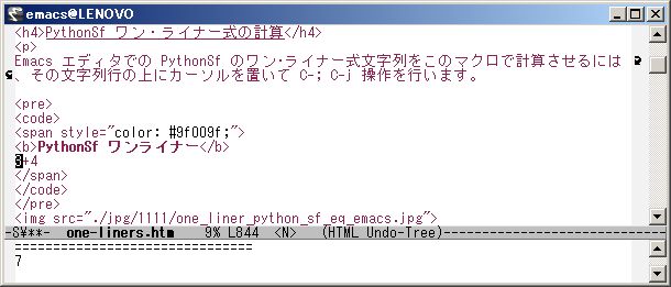
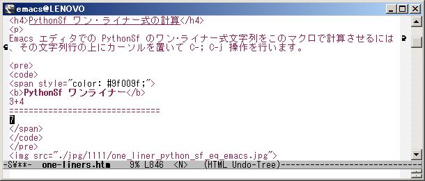
To calculate a PythonSf one-liner expression in Emacs editor, you move the cursor on the one-liner expression:the character string and operate keys:"C-;C-j".
PythonSf one-liner
3+4
===============================
7
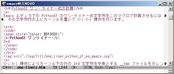
The operation C-; C-j makes a file:__tmp that contains "3+4" string, in current directory. And execute "python -u -m sfPP -fl __tmp" command string to it and execute pre-processed lines. Emacs display the computed result in the echo arear at the bottom of Emacs editor. At the same time Emacs yanks the resulted strings which OS returned through CUI.
If you want to execute a PythohSf one-liner with the PythonSf Open version, then you should operate the C-, C-j key operation.
If you want to write down the calculated result in the text, you should operate "C-y":yank.
PythonSf is upper compatible with Python, so you can execute Python one-liners with C-; C-j operation. Move the cursor on a Python one-liner code and do the C-; C-j key operation. So Emacs will execute the one-liner as below.
PythonSf one-liner
import tarfile as tr; tr.open('pycrypto-2.0.1.tar.gz', 'r').extractall()
IOError:You may use nonexistent variable name:[Errno 2] No such file or directory: 'pycrypto-2.0.1.tar.gz'
By the way, it is below 10 lines where we implement the Emacs macro for C-; C-j operation.
pysf.el function for PythonSf one-liners
(defun ExecPySf_1liner()
    "Evaluates the current line in PythonSf, then copies the result to the clipboard."
    (interactive)
    (write-region (__getLineOmittingComment) (line-end-position) "__tmp" nil)

    (let ((strAt
             (shell-command-to-string "python -u -m sfPP -fl __tmp" )
         ))
        (message strAt)
        (kill-new strAt)))
Additionaly we show the C-, C-j corresponding macro code which are called with PythonSf Open version one-liners.
pysf.el function for open version PythonSf one-liners
(defun ExecPySfOp_1liner()
    "Evaluates the current line in PythonSf, then copies the result to the clipboard."
    (interactive)
    (write-region (__getLineOmittingComment) (line-end-position) "__tmp" nil)

    (let ((strAt
             (shell-command-to-string "python -u -m sfPPOp -fl __tmp" )
         ))
        (message strAt)
        (kill-new strAt)))
You can customize this short Emacs macro easily if you cant accept these operations and actions.
the pre-processor, a __tmp file and a _tmC.py fileEmacs macro:pysf.el generates a __tmp file in a current directory with the C-; C-j or C-, C-j operation and executes "python -u -m sfPP -fl __tmp" or "python -u -m sfPPOp -fl __tmp" commands. Then it pre-processes the __tmp file and executes the python code lines which are generated by the pre-processor. The python code lines are save at the _tmC.py file in the current directory at the same time. PythonSf does not directly execute the _tmC.py file. PythonSf generates the _tmC.py file to debug it. If you want more particular trace information, you should execute the _tmC.py file. If you want single step traces. then do "python -m pdb _tmC.py"
pysf.el macro can also execute OS commands under the cursor, operating C-; C-a as below.
dir command string
dir cl*.pvl
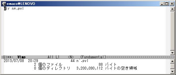
You might not be approval for just doing dir command in Emacs editor, but please think that it can execute any commands (or executable files with parameters at Windows). It can do many things, For example do ;a key operation in Emacs after moving the cursor on the below string. It will open the byte_of_vim_v051 pdf file just at the 10th page. If you modify the page parameter 10 and file name, you can open the file at the page that you want.
command starting Acrobat assigning a page number
C:"\Program Files (x86)\Adobe\Reader 9.0\Reader\AcroRd32.exe" /A page=10 D:\utl\vim73\byte_of_vim_v051.pdf
By the way, Exc_command() Emacs macro executes OS commands. If you interest it or want to customize it then refer to pysf.el file.
The upper command, which opens a pdf, file doesn't require a return value. But you can't edit Emacs while opening the pdf file because Emacs executes the opening command as a child process of Emacs. To avoid this, please do C-; Cf operation in Emacs if you are using Windows OS. Emacs macro:Exec_start() executes commands adding "start" string at Windows OS.
If you execute "start fileName" at Windows OS, then OS executes an application programm that are associated with the filename extension using the filename as a command parameter. Applying this, you might operate computers more conveniently. For example you move the cursor on URL string in Emacs and do the key operation C-; C-f then Windows OS executes the default brauser with the URL as below.
C-; C-f operation is useless at Linux. Because there is no functions that relate extensions to applications. If you want to execute OS commands concurrently, please add ; to OS command strings.
C-; C-f operation on a URL string i.e start execution
http://www.nhk.or.jp/daily/english/
You can write a comment to a one-liner in the left side untill ";;":head side for Emacs one-liner execution macros.
comment + ;; + a string of a PythonSf expression
PythonSf expression displaying a sin function graph;;plotGr(sin, 0,2pi)
Why we insist on putting a comment to head side? Though, in a PythonSf expression, we can put a comment after "#". Because we can't recognize the comment at a glance, if the PythonSf expression become long. We encounter same problems for long OS commands or URL strings. So pysf.el one-liner macro recognize a line head comment till ";;" by assuming it as delimeter. For example, move the cursor on the below URL and do C-; C-f key operation then OS make a default browser go to a web page where you can download the news voice file ro calculate a PythonSf expression.
comment + ;; + URL string
NHK English news;;http://www.nhk.or.jp/nhkworld/english/radio/program/index.html
Kennedy: We Choose to go to the Moon;;http://www.youtube.com/watch?v=g25G1M4EXrQ

comment + ;; + PythonSf expression string
comment for a PythonSf expression;;3+4
pysf.el macros can compile and execute a block code of Python or C or any other programming languages.
Block lines at pysf.el means lines between //@@ and //@@@ strings as blow. Macro of pysf.el executes or compiles the block.
a block for pysf.vim
//@@
    ・
  block lines
    ・
//@@@
If you want to calculate a number of PythonSf expressions in a block but to calculate in a one-liner, please do the next things.
Then pysf.el macro writes down lines between //@@ and //@@@ to __tmp file in current directory and executes python -u -m sfPP -fs __tmp. Then the pre-processor transforms the __tmp file to _tmC.py that Python can deal with. After that it executes "python -u _tmC.py".
PythonSf block
//@@
# 07.11.26 beer barrel form pulley
# width = 5 meter, hieght = 1meer,  depth 1 meter,

#import sf
import pysf.sfFnctns as sf

N, M =20,5
dctUpper={}
dctLower={}
for pos, index in zip(sf.masq([-2.5,N+1, 5.0/N],[-0.5,M+1, 1.0/M]), sf.mrng(N+1,M+1) ):
    dctUpper[index] = (pos[0], 1, pos[1])
    dctLower[index] = (pos[0],-1, pos[1])

N, M = 10,5
dctLeft ={}
dctRight ={}
for (theta, z), index in zip(sf.masq([sf.pi/2, N+1, -sf.pi/N], [-0.5, M+1, 1.0/M])
                            ,sf.mrng(N+1,M+1) ):
    dctRight[index] = [2.5+sf.cos(theta), sf.sin(theta),z]
    dctLeft[index] = [-2.5-sf.cos(theta), sf.sin(theta),z]


sf.renderFaces(dctUpper)
sf.renderFaces(dctLower)
sf.renderFaces(dctLeft)
sf.renderFaces(dctRight)

dctLeft ={}
dctRight ={}
N=40
for (theta, z), index in zip(sf.masq([sf.pi, N+1, -2*sf.pi/N], [-0.5, M+1, 1.0/M])
                            ,sf.mrng(N+1,M+1) ):
    dctRight[index] = [2.5+(2-sf.cosh(z))*sf.cos(theta), (2-sf.cosh(z))*sf.sin(theta),z]
    dctLeft[index] = [-2.5-(2-sf.cosh(z))*sf.cos(theta), (2-sf.cosh(z))*sf.sin(theta),z]

sf.renderFaces(dctLeft, blMeshOnly=True, meshColor=sf.red)
sf.renderFaces(dctRight, blMeshOnly=True, meshColor=sf.red)
//@@@
By the way Emacs macro:ExecSf_Bloc() executes the PythonSf block expressions. If you are interested to it, please refer it in pysf.el file.
The upper PythonSf block expressions draws a 3D belt conveyer graphic.
By the way the radius of the pulleys in the belt conveyer is bigger at the center than at the edges. It preserve the belt in center although it may oppose your intuition.
Adversely if you make the center of th pulley nallow, then the conveyer belt will be pulled to one of the edges of the pulley and the conveyer will be destroyed.
PythonSf block equations
//@@
# 07.11.26
# width = 5 meter, hieght = 1meer,  depth 1 meter,

#import sf
import pysf.sfFnctns as sf

N, M =20,5
dctUpper={}
dctLower={}
for pos, index in zip(sf.masq([-2.5,N+1, 5.0/N],[-0.5,M+1, 1.0/M]), sf.mrng(N+1,M+1) ):
    dctUpper[index] = (pos[0], 1, pos[1])
    dctLower[index] = (pos[0],-1, pos[1])

N, M = 10,5
dctLeft ={}
dctRight ={}
for (theta, z), index in zip(sf.masq([sf.pi/2, N+1, -sf.pi/N], [-0.5, M+1, 1.0/M])
                            ,sf.mrng(N+1,M+1) ):
    dctRight[index] = [2.5+sf.cos(theta), sf.sin(theta),z]
    dctLeft[index] = [-2.5-sf.cos(theta), sf.sin(theta),z]


sf.renderFaces(dctUpper)
sf.renderFaces(dctLower)
sf.renderFaces(dctLeft)
sf.renderFaces(dctRight)

dctLeft ={}
dctRight ={}
N=40
for (theta, z), index in zip(sf.masq([sf.pi, N+1, -2*sf.pi/N], [-0.5, M+1, 1.0/M])
                            ,sf.mrng(N+1,M+1) ):
    dctRight[index] = [2.5+sf.cosh(z)*sf.cos(theta), sf.cosh(z)*sf.sin(theta),z]
    dctLeft[index] = [-2.5-sf.cosh(z)*sf.cos(theta), sf.cosh(z)*sf.sin(theta),z]

sf.renderFaces(dctLeft, blMeshOnly=True, meshColor=sf.red)
sf.renderFaces(dctRight, blMeshOnly=True, meshColor=sf.red)

thetaS = 2.05117740593
#Z0 = 0.48121182506 # real value
Z0 = 0.35   # exagerated value
lstRear =[(2.5+sf.cosh(0.5)*sf.cos(thetaS),1,-0.5), (2.5, sf.cosh(-Z0), -Z0)]
lstFront =[(2.5+sf.cosh(0.5)*sf.cos(thetaS),1,0.5), (2.5, sf.cosh(Z0), Z0)]
N=30
for theta in sf.arSqnc(sf.pi/2, N+1, -sf.pi/N):
    lstRear.append( (2.5+sf.cosh(Z0)*sf.cos(theta), sf.cosh(-Z0)*sf.sin(theta),-Z0) )
    lstFront.append( (2.5+sf.cosh(Z0)*sf.cos(theta), sf.cosh(Z0)*sf.sin(theta),Z0) )

sf.plotTrajectory(lstRear, blAxis=False)
sf.plotTrajectory(lstFront, blAxis=False)
//@@@
It is a hard work to draw up 3D graphs like upper ones using drawing software like Microsoft Word. If you are with math and science majors, you might more easily draw them with PythonSf expressions.
You can also execute Python codes between //@@ and //@@@, doing ctrl+; ctrl+p key operation in Emacs editor in the same manner as upper PythonSf block executions.
Python block execution
//@@
#from;;http://www.daniweb.com/forums/thread113274.html
#from TurtleWorld import *
#TurtleWorld()
import turtle as t

def Koch(length):
    if length<=2 :
        t.forward(10*length)
        return

    Koch(length//3)
    t.left(60)
    Koch(length//3)
    t.right(120)
    Koch(length//3)
    t.left(60)
    Koch(length//3)

t.setpos(-300,10)
Koch(60)
t.exitonclick()
In addition PythonSf is upper compatible with Python, so you can execute the upper Python block codes as a block of PythonSf expression and you can also execute the upper turtle program by ;k operation It will draw the same Koch curve. It will elapse more CPU time to pre-process the codes although you will not be aware of the time difference at a commercial version of PythonSf. At a evaluation version of PythonSf, there is a 5 sec delay and you will be aware the differnece of elapsed time.
By the way Emacs macro:ExecPy_Bloc() executes the Python block codes. If you are interested to it, please refer it in pysf.el file.
You can compile,link and execute any language, continuing execution of string lines which is written just after a block. We have assigned this to ctrl+; ctrl+e key operation.
If you do the ctrl+; ctrl+e key operation, putting cursor in a code block between //@@ and //@@@, then pysf.vim macro:Exec_BlockCntn() will do below things.
If you had written down a copy command and a compile command as //copy __temp ... //gcc ..., in __temp file Exec_BlockCntn() macro writes the code beteween //@@ and //@@@ and copy and comple as a below example.
continuing execution of command with a block code: compile and execute C programm
//@@
//06.01.28  test valarray sum <== OK
#include &;t;valarray>
#include &;t;iostream>   // iostream cannot co-exist with systemc.h
using namespace std;

int main()
{
    valarray<int> vlrInAt(5);  // size 5 vararray initialize by 0
    vlrInAt[0]=1;
    vlrInAt[1]=2;
    vlrInAt[2]=3;
    vlrInAt[3]=4;
    vlrInAt[4]=5;

    cout << vlrInAt.sum() << endl;
    return 0;
}
//@@@
//copy __temp a.cpp /y
//g++ a.cpp  -O0 -g
//a
You can write any string lines after "//@@@" with ctrl+; ctrl+e key operation:continuing execution of command with a block code. If you want to execute block codes with Haskell, you might just write down as below.
continuing execution of command with a block code: compile and execute C programm
//@@
data Variables = C Char | S String | I Int | Iex Integer | D Double | F Float
data VarList a = VarX a [Variables]

instance Show Variables where
    show (C ch)  = "C "   ++ show ch
    show (S str) = "S "   ++ show str
    show (I m)   = "I "   ++ show m
    show (Iex n) = "Iex " ++ show n
    show (D o)   = "D "   ++ show o
    show (F p)   = "F "   ++ show p

instance Show a => Show (VarList a) where
    show (VarX x y) = "Var " ++ show x ++ " " ++ show y

x = VarX 11 [(Iex 21), (S "fd"), (C 'a')]

main = do
    print x
//@@@
//copy __temp temp.hs /y
//D:\lng\Haskell\ghc6121\bin\runghc.exe temp.hs

Var 11 [Iex 21,S "fd",C 'a']
You can execute upper Haskell program even without setting PATH environment variable becuase the upper example executes Haskell with the full path file name.
Continuing execution of commands with a block code is convenient for execution of test program codes which are so many and small. If you would have these small test code files by hundreds, You couldn't manage them. But you can put the codes in big one file. You would leave compile/liner options too in the big file. You can rerun each of the codes any time and a number of time just moving the cursor on one of the code block and doing the key operation ctrl+; ctrl+e in Emacs editor.
By the way there is no error handlings in Exec_BlockCntn() code. That should be fixed up. But even the current Exec_BlocnTntn() is sufficiently convenient. So we make a test exhibition of Exec_BlockCntn()
You could input kanji characters of greek letters or ∂∇□△ symbols using Windows IME. But it is bother to do on/off operations of IME in the typing actions of expressions. We have implemented Emacs macro:ConvertAlpbt2Greek() that help out to input the greek/symbol characters
We have slightly extended Python syntax to resemble PythonSf expression to memo writing mathematical expressions. You might come across PythonSf expressions that you can't understand, if you don't understand the extended parts of the syntax. PythonSf beginner should read this chapter through.
Product operators are abbreviated in general at Mathematics. Alsot PythonSf take over the abbreviation.
We implement PythonSf aiming to resemble daily PythonSf expression to memo writing matmematical expressions. So we intervene in syntax analysys proces using a pre-processor to abbreviate the product operators as below.
PythonSf one-liners
a,b=3,4; 2 a b
===============================
24

a,b=3,4; 2a + 3b
===============================
18

a,b=3,4; 2(a+b)
===============================
14

a,b=3,4; a (a+b)
===============================
21

PythonSf one-liner missusing the abreviation of product operators
a,b=3,4; ab
name 'ab' is not defined at excecuting:ab

a,b=3,4; a(a+b)
'int' object is not callable at excecuting:a(a+b)
Please notice that you can't write expressions as ab or a(a+b) for compliance with Python syntax. "ab" mmeans a variable ab not a expression a*b at Python syntax. "a(a+b)" means a function "a" with a parameter "a+b" not a expression a*(a+b).
Generally "^" is used for exponentiation operator. "**" operator is used only in programming. On the other hand "^" operator means bit exor in Python.
We preffered to resemble PythonSf expression to memo writing mathematical expressions than to maintain Python syntax. Python use \^ for bit exor operator. Definitely you can also use ** operator as a exponentiation operator at PythonSf expressions. We show up examples as below.
PythonSf one-liner
2^4, 2\^4, 2**4
===============================
(16, 6, 16)
Though we sait that PythonSf was upper compatible with Python, there are few of parts that are not compatible with Python. In Python you can calculate "sin (pi/3)" inserting space, but it means sin*(pi/3) in PythonSf as at ^ operator. But you might not use bit exor operator less than once a year. You need no space between sin and (pi/3). It shoud be allowed to say tha PythonSf is compatible with Python, if the imcompatible exceptions are limited in few parts.
It is desirable that you can write PythonSf expressions shortly as far as possible. There are many implicit assumptions. For example "x" "y" means given variables and &quto;x+y" means a addition of variables i.e. a function of two variables. But at programming, you must write declaring statement of x,y to avoid undefined variable erros.
You can avoid the undefined erros, if you have assigned some instances to x,y. But it wrongly affect Python codes to assign some objects ot very short labels of x,y.
We have allowed PythonSf labels to add backquote(s) at head or tail of them. We have extended PythonSf namespace adding backquote and enable to use short mathematical labels that are not in the existing Python namespace.
For example, to "`X" we have assigned a instance of a identical function class that has four operations methods and exponentiation operation method. So you can use "`X^2+3`X+1" as a quadratic function as below.
PythonSf one-liners
(`X^2+3`X+1)(1)
===============================
5

(`X^2+3`X+1)(2)
===============================
11

x=`X; (x^2+3x+1)(3)
===============================
19
To "`Y" we have assigned a instance of a identical function class that has four operations methods and exponent operation method and a method picking up the 2nd argument from parameters. So you can use " `X^2+3`Y" as a quadratic function of 2 variables as below.
PythonSf one-liners
(`X^2+3`Y+1)(1,2)
===============================
8

sqrt(`X^2+3`Y+1)(1,2)
===============================
2.82842712475
We use ~[...] syntax to indicate vectors or matrices as below.
PythonSf one-liners
~[1,2,3]    # float value vector
===============================
[ 1.  2.  3.]
---- ClTensor ----

~[1,2,3+4j]    # complex value vector
===============================
[ 1.+0.j  2.+0.j  3.+4.j]
---- ClTensor ----

vc=~[1,2,3]; vc+[4,5,6]    # vector add
===============================
[ 5.  7.  9.]
---- ClTensor ----

vc=~[1,2,3]; vc [4,5,6]    # vector inner product
===============================
32.0

~[ [1,2],[3,4] ]           # matrix
===============================
[[ 1.  2.]
 [ 3.  4.]]
---- ClTensor ----

mt,vc=~[[1,2],[3,4]],~[5,6]; mt vc   # product of matrix and vector
===============================
[ 17.  39.]
---- ClTensor ----

mt=~[[1,2],[3,4]]; 1/mt, mt^-1   # inverse of matrix
===============================
(ClTensor([[-2. ,  1. ],
           [ 1.5, -0.5]]),
 ClTensor([[-2. ,  1. ],
           [ 1.5, -0.5]]))

# a generation of a ClTensor matrix instance from a matrix dictionary object
dct={(0,0):1,(0,1):2,(1,0):3,(1,1):1}; ~[dct]
===============================
[[ 1.  2.]
 [ 3.  1.]]
---- ClTensor ----
We assign a floating type vector or matrix by default because it both of integer type and floating type one bring about same result values. Adversely dividing operation of a integer type vector or matrix bring about 0 values after the decimal points.
If you want to use vectors or matrices other than floating type, please ust ~[..., type] syntax adding type parameter at the tail posiion.
PythonSf one-liner
~[1,2,3, int]   # int type vector
==============================
[1 2 3]
---- ClTensor ----
If you set user defined type like as oc.BF, you can operate that type vectors or matrices.
PythonSf one-liners
~[1,0,1, oc.BF]     # oc.BF:Bool Filed type vector
===============================
[1 0 1]
---- ClFldTns:<class 'pysf.octn.BF'> ----

mt,vc=~[[1,1,0],[1,1,1],oc.BF],~[1,0,1, oc.BF]; mt vc     # product of Bool Type matrix and vector
===============================
[1 0]
---- ClFldTns:<class 'pysf.octn.BF'> ----

~[1,2,3, oc.BF]     # oc.BF:Bool Filed type vector
===============================
[1 0 1]
---- ClFldTns:< class 'pysf.octn.BF'> ----

class Cl(int):pass; ~[1,2,3, Cl]    # user defined type
===============================
[1 2 3]
---- ClFldTns:&;t;class 'pysf.sfPPrcssr.Cl'> ----
PythonSf ~[...] syntax generates instances of ClTensor class or ClFldTns class, not instances of ndarra in Numpy. Because it makes us to describe multiplication and division of vectors or matrices multiply as like as the ways of integer or float. So that multiplication of the ClTensor or ClFldTns instances is multiplication of a matrix and vector or matrix and matrix. Multiplication of the ClTensor or ClFldTns vectors is inner product. At ClTensor or ClFldTns, division of vector over vector become a error. Meanwhile at ndarray, multiplications means multiplications of each element. You well be puzzled at first time. Please notice this.
PythonSf one-liner
# Multiplication for vectors: inner product at PythonSf
~[1,2,3] ~[4,5,6]
===============================
32.0

PythonSf one-liner
~[1,2,3]/ ~[4,5,6]
Traceback (most recent call last):
  File "D:\lng\Python26\lib\runpy.py", line 122, in _run_module_as_main
    "__main__", fname, loader, pkg_name)
  File "D:\lng\Python26\lib\runpy.py", line 34, in _run_code
    exec code in run_globals
  File "D:\my\vc7\mtCm\sfPP.py", line 2, in
    pysf.sfPPrcssr.start()
  File "pysf\sfPPrcssr.py", line 2722, in start
    __execLine( (" ".join(sys.argv[1:])).strip() )
  File "pysf\sfPPrcssr.py", line 2345, in __execLine
    valStt = eval(ustConvertedAt, globals(), locals() )
  File "", line 1, in
  File "pysf\sfFnctns.py", line 547, in __truediv__
    return self.__mul__(ag.inv())
  File "pysf\sfFnctns.py", line 492, in inv
    return copy.deepcopy(self.m_inv)
  File "pysf\sfFnctns.py", line 909, in __getattr__
    self.__dict__['m_inv'] = ClTensor(sl.inv(self))
  File "D:\lng\Python26\lib\site-packages\numpy\linalg\linalg.py", line 423, in inv
    return wrap(solve(a, identity(a.shape[0], dtype=a.dtype)))
  File "D:\lng\Python26\lib\site-packages\numpy\linalg\linalg.py", line 290, in solve
    _assertRank2(a, b)
  File "D:\lng\Python26\lib\site-packages\numpy\linalg\linalg.py", line 134, in _assertRank2
    two-dimensional' % len(a.shape)
numpy.linalg.linalg.LinAlgError: 1-dimensional array given. Array must be             two-dimensional

PythonSf one-liner
# division for vectors: inner product at PythonSf
vA,vB = np.array([1,2,3]),np.array([4,5,6]); vA/vB
===============================
[ 0.25  0.4   0.5 ]

PythonSf one-liner
# division for vectors: division for each elements at Numpy
np.array([1,2,3]) np.array([4,5,6])
===============================
[ 4 10 18]

np.array([1,2,3])/np.array([4,5,6])
===============================
[ 0.25  0.4   0.5 ]
In addition we add a "---- ClTensor ----" string if calculation results are a vector or matrix which element is integer or float or complex. We add something like "---- ClFldTns:< class 'pysf.octn.BF'> ----" string if calculation results are a vector or matrix which element is not integer and float and complex. We add no string if calculation results are numpy.ndarray instances. We show up examples below.
an expression of ClTensor instances
===============================
returned value
---- ClTensor ----


an expression of ClFldTns instances
===============================
returned value
---- ClFldTns:< class 'pysf.octn.BF'> ----

an expression of np.ndarray instances
===============================
returned value
# There is no explicit type information
PythonSf one-liners
σx,σz=~[[0,1],[1,0]], ~[[1,0],[0,-1]]; σx σz
===============================
[[ 0. -1.]
 [ 1.  0.]]
---- ClTensor ----

σx,σz=~[[0,1],[1,0]], ~[[1,0],[0,-1]]; σx+σz
===============================
[[ 1.  1.]
 [ 1. -1.]]
---- ClTensor ----
In addition to Greek characters, you can use special kanji symbols "∇□∂△" which are frequently used in daily calculations. Particularly the differential symbol:∂ is conveniently in heavy usage as below.
PythonSf one-liners
# numerical differentiation
∂x(`X^2+2`X+3)(2)
===============================
6.0

# symbolic differentiation
ts(); ∂x(`x^2+2`x `y+3)
===============================
2*x + 2*y

# Jacobian numerical differentiation
∂J(`X^2+`Y^2, 2)(1,2)
===============================
[ 2.  4.]
---- ClTensor ----
PythonSf use Greek kanji character:λ to lambda expressions, becuase it wins an advantage over visibility and lambda expressions are frequently used. Herewith you can use λ expression as in computer science textbooks as below. In return to the advantage, you can't use the variable which is only one character:λ
PythonSf one-liners
f=λ x:sin(x)+2cos(x); f(pi/2)
===============================
1.0

# Using let statement utilizing a default parameter in a λ expression.
# The default parameter:y=sin(x)+2cos(x) might be considered as a let statement.
# You cant change the y value.
f=λ x:(λ y=sin(x)+2cos(x): y+y^2)(); f(pi/2)
===============================
2.0

# You can't assign a value to λ label. Becuase λ is lambda syntax.
λ=3; 2λ
invalid syntax (, line 1) at excecuting:lambda=3
Lambda expressions in Python resemble to lambda expression in computer science textbooks. You can model the natural number using Church number as below.
PythonSf one-liners
# 2 at Church number
Z='1';S =λ s:s+'1';(λ s:λ z:s(s(z)))(S)(Z)
===============================
111

# 2 + 3 at Charch number
Z='1';S =λ s:s+'1';(λ s:λ z:s(s(  s(s(s(z))) )))(S)(Z)
===============================
111111
You can diffine infix operators:~~, ~^, ~+, ~-, ~*, ~/, ~%, ~&, ~|, ~== for yourself. Please note that the kind of the priority of the user operators is only one:maximum only. So you might control the priority by parentheses.
For example, we assigned nearlyEq(..) function to ~== extended user operator. So you can calculate as below.
PythonSf one-liners
(3.3pF`) ~== (3.300001pF`)
===============================
True

(3.3pF`) ~== (3.30001pF`)
===============================
False

~[1, 2] ~== [1, 2.000001]
===============================
True

~[1, 2] ~== [1, 2.00001]
===============================
False
The pre-processor of PythonSf imports sfFnctns.py module before calculations. So PythonSf has imported a lot of basic mathematical objects as basic numeric functions:exp, sin, cos, tan, sinh, cosh, tanh, arcsin, arccos, arctan, log10, sqrt and athers to the global name space. So you can calculate the basic numeric functions without importing math. You can do almost all the calculations that normal scientifc calculator do as below.
PythonSf one-liner
tan(pi/3)
===============================
1.73205080757
Though we had used extended variable as `X, you can use variables which are added multiple single quate(s) in head or tails, because PythonSf intervene in syntax analysis process. It is allowed that Python syntax works with short mathematical expressions according to mathematical conventions because of extended name space and customizing i.e. assigning Python objects to short labels.
Let look more concretely. If PythonSf pre-processor founds a variable lable that starts with "`", it adds "k__bq_" at the head of the label and adds "__" at the tail of the label. For example the pre-processor transforms "`X" to k__bq_X__. And we have assigned the short label a identical function that is a Python object and allowed four and exponent operations. So you can write short expressions as "`X^2+1" and others.
It is desirable to write mathematical expressions shortly as far as possible. So the expression are written under many implicit assumptions. In the field of mathematics "X" means a unkown variable. In the field of physics "h" means Planck constant and "c" means the light velocity. But it is crazy to assign short variable names Python objects as of identical function, Planch constant, light velocity, because they might conflict with Python codes in some way.
To avoid this problem, we extended the name space adding one or more back quotes at head or tail. Assigning a identical function or Planck constant or others to the extended labels, we enabled to write short calculatable memo writing expression that assumes implict assumptions at the field of mathematics or physics or others.
By the way we use a naming conventions adding a back quotes at tail for physical units or constants.
In addition we also use back quotes to notate upper or lower indexes of tensor as Γ``_[i,j,k]. For this example i,j is upper index and k is lower index. You migh say that the back quotes are int in tail at Γ``_. Please regard that _:underscore as not included at tails of name string when more appropriate.
There are many implicit assumptions for fields of each expertise at each users. You may use different assumptions for each directories as the cases.
So we use pysf\customize.py file for global implicit assumptions. Adversely you can use sfCrrntIn.py file in current directory for local implict assumptions. PythonSf does "from pysf.customize import *" and does "from sfCrrntIni import *" if there is a sfCrrntIn.py file in the current directory.
There are customize.py and sfCrrntIni.py files in distributions of PythonSf. We have defined phyisical units as of &"kg`" or variables as of "`X". In addition, we have defined pure imaginary number unit:"`i", Pauli matrix:"`σx `σy `σz" and others in customize.py. We also have defined ratianal unit number:"`1r" in ts() function on customize.py. You can calculte expressions as below.
PythonSf one-liners
exp(2pi `i/3)
===============================
(-0.5+0.866025403784j)

# addition of oc.BF Bool value vectors
~[`1,`0,`1]+[`1,`1,`1]
===============================
[0 1 0]
---- ClFldTns:< class 'pysf.octn.BF'> ----

`σx + 2`σy
===============================
[[ 0.+0.j  1.-2.j]
 [ 1.+2.j  0.+0.j]]
---- ClTensor ----

# calculation of exponential matrix
t,mt=0.1, `σx + 2`σy; expm(`i t mt)
===============================
[[ 0.97510399+0.j          0.19833750+0.09916875j]
 [-0.19833750+0.09916875j  0.97510399+0.j        ]]
---- ClTensor ----

# series of rational number
ts(); [`1r/(k+1) for k in range(10)]
===============================
[1, 1/2, 1/3, 1/4, 1/5, 1/6, 1/7, 1/8, 1/9, 1/10]

ts(); sum( [`1r/(k+1) for k in range(10)] )
===============================
7381/2520
We also have defined rank 3 Levi-Civita tensor:"εL, difirentiating function:"∂x",Laplace operator unary polynomial:"`s" and others, so you can calculate expressions using these Python objects as below.
PythonSf one-liners
`εL # Levi-Civita tensor
===============================
[[[ 0. 0. 0.]
[ 0. 0. 1.]
[ 0. -1. 0.]]
[[ 0. 0. -1.]
[ 0. 0. 0.]
[ 1. 0. 0.]]
[[ 0. 1. 0.]
[-1. 0. 0.]
[ 0. 0. 0.]]]
---- ClTensor ----
a,b=~[1,2,3],~[4,5,6]; -a `εL b # outer product by Levi-Civita tensor
===============================
[-3. 6. -3.]
---- ClTensor ----
a,b=~[1,2,3],~[4,5,6]; np.cross(a,b) # outer product by Numpy
===============================
[-3. 6. -3.]
∂x(`X^2+1)(1) # differential value of x^2+1 at 1
===============================
2.0
∂J(~[`X+`Y, `X `Y], 2)(1,2) # Jacobian of ~[x+y,x y] field at [1,2]
===============================
[[ 1. 1.]
[ 2. 1.]]
---- ClTensor ----
1/(`s+1) ( (`s+2) +1/(`s+3)) # calculate Laplace operator expression
===============================
2
1 s + 5 s + 7
-------------
2
s + 4 s + 3
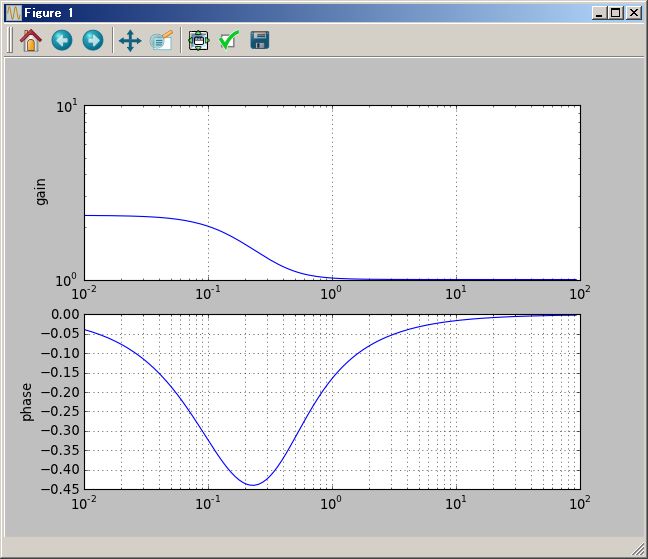
# Bode plot
(1/(`s+1) ( (`s+2) +1/(`s+3))).plotBode(0.01Hz`,100Hz`)
In sfCrrntIni.py we have defined Z2,Z3,Z4,Z5,Z7 that are Zp(N) where N is 2,3,4,5,7. There is in global variables, so you can use Z2,Z3,Z4,Z5,Z7 freely in Pythonsf expressions as blow.
PythonSf one-liners
# Z3 行列
~[range(2*2), Z3].reshape(2,2)
===============================
[[Z3(0) Z3(1)]
 [Z3(2) Z3(0)]]
---- ClFldTns:< class 'sfCrrntIni.Z3'> ----

# Z3 行列の逆行列
mt=~[range(2*2), Z3].reshape(2,2); mt^-1
===============================
[[Z3(0) Z3(2)]
 [Z3(1) Z3(0)]]
---- ClFldTns:< class 'sfCrrntIni.Z3'> ----

# Z3 行列どうしの積
mt=~[range(2*2), Z3].reshape(2,2); mt mt^-1
===============================
[[Z3(1) Z3(0)]
 [Z3(0) Z3(1)]]
---- ClFldTns:< class 'sfCrrntIni.Z3'> ----
You should customize "customize.py" or "sfCrrntIni.py& by yourself at your convenience. The contents of them are only Python codes, so you can freely change them according to your need.
You can make a file variable of a picklable instance. In current directory, this file variable is made as a file that extensions is "pvl". In other words using OOP terms, you can serialize calculated picklable results and can reuse them anytime. You can write the file variable by ":=" and can read it by "=:" The function of file variable is resembling the function of sfCrrntIni.py
As we show up below, "tmp:=3+4" makes tmp.pvl file in current directory. You can read the "tmp.pvl" file as by "=:tmp; tmp/2". ":=tmp" reads tmp.pvl file in current directory and set the value to tmp global variable of Python, then you can calculate expression which contain tmp variable.
PythonSf one-liner
tmp:= 3+4
===============================
7
dos command
dir tmp.pvl
D:\my\vc7\mtCm>dir tmp.pvl
 Volume in drive D is ?????
 Volume Serial Number is 4CBC-BC86

 Directory of D:\my\vc7\mtCm

2012/06/15  11:16                42 tmp.pvl
               1 File(s)             42 bytes
               0 Dir(s)  12,429,426,688 bytes free

dos command
type tmp.pvl
# python object printed out by pprint
7

PythonSf one-liner
# read tmp.pvl and halve it
=:tmp; tmp/2
===============================
3.5
We show up most practical examples of file variables. There are X32.pvl,X64.pvl,X28.pvl, Px32.pvl,Px64.pvl,Px128.pvl files that are position operators of arear [-1,1] and momentum operators of arear [0,2pi]. These are used for Heisenberg's matrix mechanics. For example we show X32 below.
PythonSf one-liner
P,X=:Px32,X32; X
===============================
[[-0.96875  0.       0.      ...,  0.       0.       0.     ]
 [ 0.      -0.90625  0.      ...,  0.       0.       0.     ]
 [ 0.       0.      -0.84375 ...,  0.       0.       0.     ]
 ...,
 [ 0.       0.       0.      ...,  0.84375  0.       0.     ]
 [ 0.       0.       0.      ...,  0.       0.90625  0.     ]
 [ 0.       0.       0.      ...,  0.       0.       0.96875]]
---- ClTensor ----
You can describe a Hamiltonian matrix as a polynomial made of the position matrix and momentum matrix, so you can calculate the equations those are explained in textbooks of quantum mechanics. For example you can write down a Hamiltonian of harmonic oscillator as below
PythonSf one-liner
P,X=:Px64, X64; H=P^2+X^2;          H
===============================
[[ 4.25805908 +8.32667268e-17j  1.99678801 +9.80959047e-02j
   0.49679034 +4.89295777e-02j ...,  0.21901645 -3.24880216e-02j
   0.49679034 -4.89295777e-02j  1.99678801 -9.80959047e-02j]
 [ 1.99678801 -9.80959047e-02j  4.19751221 +5.55111512e-17j
   1.99678801 +9.80959047e-02j ...,  0.12179970 -2.42274668e-02j
   0.21901645 -3.24880216e-02j  0.49679034 -4.89295777e-02j]
 [ 0.49679034 -4.89295777e-02j  1.99678801 -9.80959047e-02j
   4.13891846 -5.55111512e-17j ...,  0.07680678 -1.92390964e-02j
   0.12179970 -2.42274668e-02j  0.21901645 -3.24880216e-02j]
 ...,
 [ 0.21901645 +3.24880216e-02j  0.12179970 +2.42274668e-02j
   0.07680678 +1.92390964e-02j ...,  4.13891846 +2.04697370e-16j
   1.99678801 +9.80959047e-02j  0.49679034 +4.89295777e-02j]
 [ 0.49679034 +4.89295777e-02j  0.21901645 +3.24880216e-02j
   0.12179970 +2.42274668e-02j ...,  1.99678801 -9.80959047e-02j
   4.19751221 +6.80011603e-16j  1.99678801 +9.80959047e-02j]
 [ 1.99678801 +9.80959047e-02j  0.49679034 +4.89295777e-02j
   0.21901645 +3.24880216e-02j ...,  0.49679034 -4.89295777e-02j
   1.99678801 -9.80959047e-02j  4.25805908 -8.32667268e-17j]]
---- ClTensor ----
This Hamiltonian matrix is just only an approximation of infinite one in Hilbert space. Though it is the approximation by a 64x64 matrix at most, it has properties that the harmonic oscillator has in quantum mechanics. Let start with ascending order energy eigenvalues of the Hamiltonian and a list of deference between neighboring elements.
PythonSf one-liners
# Ascending order eigenvalues of the Hamiltonian
P,X=:Px64, X64; H=P^2+X^2; eigvalsh(H)
===============================
[  0.03125000+0.j   0.09375000+0.j   0.15625000+0.j   0.21875000+0.j
   0.28125000+0.j   0.34374997+0.j   0.40625022+0.j   0.46874830+0.j
   0.53125901+0.j   0.59370001+0.j   0.65642917+0.j   0.71797533+0.j
   0.78307742+0.j   0.83758165+0.j   0.91619057+0.j   0.94962095+0.j
   1.06362868+0.j   1.07763419+0.j   1.23050560+0.j   1.23652959+0.j
   1.41810063+0.j   1.42121437+0.j   1.62625614+0.j   1.62810710+0.j
   1.85462810+0.j   1.85582224+0.j   2.10294704+0.j   2.10374776+0.j
   2.37102704+0.j   2.37156478+0.j   2.65874147+0.j   2.65908661+0.j
   2.96600288+0.j   2.96619493+0.j   3.29274974+0.j   3.29281031+0.j
   3.63887701+0.j   3.63893806+0.j   4.00435423+0.j   4.00453612+0.j
   4.38921091+0.j   4.38952113+0.j   4.79342210+0.j   4.79387721+0.j
   5.21696632+0.j   5.21759441+0.j   5.65982304+0.j   5.66066864+0.j
   6.12196967+0.j   6.12310288+0.j   6.60337666+0.j   6.60491066+0.j
   7.10399790+0.j   7.10612440+0.j   7.62374802+0.j   7.62681621+0.j
   8.16243915+0.j   8.16715679+0.j   8.71954535+0.j   8.72762234+0.j
   9.28731293+0.j   9.31657988+0.j   9.75250929+0.j  10.19014824+0.j]
---- ClTensor ----

# Differences of the eigenvalues of the Hamiltonian
P,X=:Px64, X64; H=P^2+X^2; vc=eigvalsh(H); vc=vc-shftSq(vc)
Waring: don't use assignment at last sentence.We ignore the assignment.
===============================
[  3.12500000e-02+0.j   6.25000000e-02+0.j   6.25000000e-02+0.j
   6.24999998e-02+0.j   6.25000026e-02+0.j   6.24999695e-02+0.j
   6.25002517e-02+0.j   6.24980750e-02+0.j   6.25107081e-02+0.j
   6.24410072e-02+0.j   6.27291558e-02+0.j   6.15461604e-02+0.j
   6.51020863e-02+0.j   5.45042324e-02+0.j   7.86089186e-02+0.j
   3.34303833e-02+0.j   1.14007733e-01+0.j   1.40055090e-02+0.j
   1.52871408e-01+0.j   6.02399218e-03+0.j   1.81571035e-01+0.j
   3.11374152e-03+0.j   2.05041772e-01+0.j   1.85096230e-03+0.j
   2.26521002e-01+0.j   1.19413904e-03+0.j   2.47124794e-01+0.j
   8.00725528e-04+0.j   2.67279275e-01+0.j   5.37743185e-04+0.j
   2.87176693e-01+0.j   3.45136237e-04+0.j   3.06916275e-01+0.j
   1.92040921e-04+0.j   3.26554815e-01+0.j   6.05733205e-05+0.j
   3.46066693e-01+0.j   6.10529677e-05+0.j   3.65416172e-01+0.j
   1.81887321e-04+0.j   3.84674788e-01+0.j   3.10218641e-04+0.j
   4.03900971e-01+0.j   4.55112728e-04+0.j   4.23089107e-01+0.j
   6.28094792e-04+0.j   4.42228631e-01+0.j   8.45595766e-04+0.j
   4.61301033e-01+0.j   1.13320700e-03+0.j   4.80273786e-01+0.j
   1.53399721e-03+0.j   4.99087243e-01+0.j   2.12649374e-03+0.j
   5.17623621e-01+0.j   3.06819454e-03+0.j   5.35622935e-01+0.j
   4.71764271e-03+0.j   5.52388560e-01+0.j   8.07698830e-03+0.j
   5.59690586e-01+0.j   2.92669528e-02+0.j   4.35929408e-01+0.j
   4.37638952e-01+0.j]
---- ClTensor ----
The first eigen value is 2pi h/2:2/64:3.125e-2:zero point energy. The next deference of the eigenvalues is 2pi h:4/64:6.25e-2.25e. The eigenvalues distribute on a parabolic curve, if they are near the zero point energy. But they distribute on a .. if they get away from the zero point energy. You can visualize the distribution as below.
PythonSf one-liner


P,X=:Px64, X64; H=P^2+X^2; plotGr( eigvalsh(H) )

You can also calculate a dynamic motion of a wave function by the Hamiltonian. If a initial condition is geven as a vector which has concenterd point at the 16th index, you can calculate the dynamics of the wave function including the phase and visualize the result by the below natural one-liner.
PythonSf one-liner


P,X=:Px64, X64; H=P^2+10 X^2; vc=kzrs(64); vc[16]=1; renderMtCplx( ~[ expm(`i H t) vc for t in klsp(0, 5s`)])
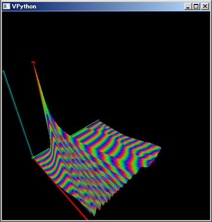
You can user customize files any number of times. So you can utilize customize files as customizing data. You can utilize picklable instances as a customizing data. But you can reuse them by re-reading them using :=. It is small time load to re-read them for PythonSf. If you write a time spending codes in customizing files, PythonSf read them for all each run time, so it will increase response time. So you can utilize PythonSf file variables as customizing data.
PythonSf has basic numeric functions:exp, sin, cos, tan, sinh, cosh, tanh, arcsin, arccos, arctan, log10, sqrt, absF these are global functions. You can use them without import any statement. In addition they can do four operations, exponentiations and functional composition as below.
PythonSf one-liner
x=pi/6; ( 2 sin cos )(x), sin(2`X)(x)
===============================
(0.8660254037844386, 0.8660254037844386)
We use ClAF class to enable four operations, exponentiation and composition. It is implemented in pysf.basicFnctns module. We make ClAF instances of Numpy exp, sin, cos, tan, sinh, cosh, tanh, arcsin, arccos, arctan, log10, sqrt.
You can customize your functions enable to do four operations, exponetiation and composition by writing codes that instantiates ClAF with your functions in customize.py or sfCrrntIni.py files. These are imported at each PythonSf run time. So you can use your functions that can do four operations, exponentiation and composition without any import statement.
We implement ClAF instances of exp, sin, cos, tan, sinh, cosh, tanh, arcsin, arccos, arctan, log10, sqrt in pysf.kNumeric module. Plese read the file, if you are interested in these functions.
In mathematical world, x,y,z mean variables. Without referring x,y,z, you can write expressions as sin(x^2), cos(2x+1), tan(x+y), exp(x^2+y^2+z^2) and others. And there meanings are clear. You can write quadratic function x^2+2x+3 without referring x.
To enable to write such expressions, We have introduced `X,`Y,`Z,`T variables these are assigned as identical functions these can do four operations, exponentiation and composition. These are assigned in customize.py file. These identical functions:`X,`Y,`Z,`T also mean to select the first,second,third and last parameter from argments. Though they are identical functions, you can write any polynomial combining them as below.
PythonSf one-liners
(`X^2+2`X+3)(2)     # quadratic function
===============================
11

(`X^2+`Y^2)(2,3)     # 2 parameter quadratic function
===============================
13

(`X^2 + `T)(2,3)    # `T picks up the last parameter 3
===============================
7

N=6; [(sin(2`X))(n/N) for n in range(N)]
===============================
[0.0, 0.32719469679615221, 0.61836980306973699, 0.8414709848078965, 0.97193790136331271, 0.99540795775176494]
In Python there are Numpy, SciPy packages these implement very big mathematical libraries. SciPy contain Numpy, SciPy has sub packages as scipy.optimize,integrate,linalg,special,signal and others these are sold as a proprietary package in Matlab. But Numpy doesn't have these packages.
But you have to use Numpy package. Because SciPy is too big and you have to wait to import it. It would be 2 second if computers are low power such as netbooks those CPU is N280. On the other hand it is 200 mili second to import Numpy even at netbooks. So PythonSf importr Numpy at every turn. But SciPy is imported when you call sy() function.
If you call sy() function, Python dose "import scipy as sy" statement. In addition, it imports below sub packages and set so,si,sl,ss,sg module labels for them. These sub packaged has below features.
PythonSf imports Numpy at every turn in pysf.sfFnctns module by "import numpy as np" statement. You can use large number of functions in Numpy package under np name-space as below.
PythonSf one-liner
# numpy.source(..) returns souce code for a function or class that is given as a parameter
np.source(fft)
In file: pysf\kNumeric.py

def fft(sqAg, n=None, axis = -1):
    """' reverse Fasst Fourier Transform
         return ClTensor array
    '"""
    import numpy.fft as fp
    return sf.krry(fp.fft(sqAg, n, axis))

===============================
None

PythonSf one-liner
# numpy.info(..) returns conpact information about a function or class that is given as a parameter
# The information is not too detailed as help(..)
np.info(np.linalg)
Core Linear Algebra Tools
-------------------------
Linear algebra basics:

- norm            Vector or matrix norm
- inv             Inverse of a square matrix
- solve           Solve a linear system of equations
- det             Determinant of a square matrix
- lstsq           Solve linear least-squares problem
- pinv            Pseudo-inverse (Moore-Penrose) calculated using a singular
                  value decomposition
- matrix_power    Integer power of a square matrix

Eigenvalues and decompositions:

- eig             Eigenvalues and vectors of a square matrix
- eigh            Eigenvalues and eigenvectors of a Hermitian matrix
- eigvals         Eigenvalues of a square matrix
- eigvalsh        Eigenvalues of a Hermitian matrix
- qr              QR decomposition of a matrix
- svd             Singular value decomposition of a matrix
- cholesky        Cholesky decomposition of a matrix

Tensor operations:

- tensorsolve     Solve a linear tensor equation
- tensorinv       Calculate an inverse of a tensor

Exceptions:

- LinAlgError     Indicates a failed linear algebra operation
===============================
None

PythonSf one-liner
# pseud-inverse of matrix
np.linalg.pinv([[1,2,3],[4,5,6]])
===============================
[[-0.94444444  0.44444444]
 [-0.11111111  0.11111111]
 [ 0.72222222 -0.22222222]]

PythonSf one-liner
# confirmation of upper result
# The multiplication with pseud-inverse is a unit matrix
np.dot([[1,2,3],[4,5,6]], np.linalg.pinv([[1,2,3],[4,5,6]]))
===============================
[[  1.00000000e+00  -4.44089210e-16]
 [  0.00000000e+00   1.00000000e+00]]
By the way, we have modified Numpy Fourier transform:fft,ifft,fftshift, eigen values or eigen vectors:eig,eigvals, exponetial/logarithm/square root of matrix:expm,logm,sqrtm, and random: rand,randn,randint,shuffle those are used frequently and changed to return ClTensor instances. You can directly use these functions as below.
PythonSf one-liners
fft([1,2,3,4])
===============================
[ 10.+0.j  -2.+2.j  -2.+0.j  -2.-2.j]
---- ClTensor ----

eig([[1,2],[3,4]])
===============================
(ClTensor([-0.37228132,  5.37228132]),
ClTensor([[-0.82456484, -0.41597356],
       [ 0.56576746, -0.90937671]]))

eigvals([[1,2],[3,4]])
===============================
[-0.37228132  5.37228132]
---- ClTensor ----

expm([[1,2],[3,4]])
===============================
[[  51.9689562    74.73656457]
 [ 112.10484685  164.07380305]]
---- ClTensor ----

sqrtm([[1,2],[3,4]])
===============================
[[ 0.55368857+0.46439416j  0.80696073-0.21242648j]
 [ 1.21044109-0.31863972j  1.76412966+0.14575444j]]
---- ClTensor ----

seed(0); rand(2,3)
===============================
[[ 0.5488135   0.71518937  0.60276338]
 [ 0.54488318  0.4236548   0.64589411]]
---- ClTensor ----

seed(0); randn(2,3)
===============================
[[ 1.76405235  0.40015721  0.97873798]
 [ 2.2408932   1.86755799 -0.97727788]]
---- ClTensor ----

seed(0); randint(10,size=[2,3])
===============================
[[5 0 3]
 [3 7 9]]
---- ClTensor ----

seed(0); shuffle(range(10))
===============================
[2, 8, 4, 9, 1, 6, 7, 3, 0, 5]
You can use SciPy package after calling sy() function as below.
PythonSf one-liner
sy(); sy.factorial(10), sy.factorial(10, True)
===============================
(array(3628800.0), 3628800L)
SciPy will be imported as sy label of the package, if you call sy() function. Function sy() alsom executes "import scipy.optimize as so","import scipy.integrate as si","import scipy.linalg as sl","import scipy.special as ss","import scipy.signal as sg" statements. Calling sy() only one time, you can use very huge amount of functions in optimize,integrate,linalg,special,signal sub packages under the lebels of so,si,sl,ss,sg.
PythonSf one-liners
sy(); so.bisect(`X^3+2`X^2-3`X-1, -10,10)   # find 0 point by bi-section method
===============================
1.19869124352

PythonSf one-liners
# double integral: integral of functio f(x,y)=x^2 + y^2 on a area in a circle with a radius of 1 from a origin
sy(); si.dblquad(`X^2+`Y^2, -1,1, sqrt(1-`X^2),-sqrt(1-`X^2) )
===============================
(-1.5707963267947727, 1.2484818956437493e-08)
# 1.2484818956437493e-08 in right side is a estimated accidental error

PythonSf one-liners
sy(); sl.sinm(`σx)         # sinm(x) == x - x^3/3! + x^5/5! - ...
===============================
[[ 0.          0.84147098]
 [ 0.84147098  0.        ]]
# Attention! Universal functions in SciPy return ClTensor instances if you give ClTensor instances parameter.
# But there are some functions these are not ufunc and doesn't return ClTensor instance as sl.sinm, even though you give a ClTensor instance parameter.

PythonSf one-liners
sy(); ss.zeta(3,0)          # special function ζ(..)
===============================
1.79769313486e+308
"info functions in Numpy" is very convenient. It prints more compact information than "help() function" and just only np.info(..)'s information is sufficient frequently. You can use np.info(..) for every Python object as of package, module, class, function or a instance which have document strings. "np.info(..)" should be used more frequently without limiting in PythonSf.
PythonSf ワンライナー
np.info(set)
 set()

set() -> new empty set object
set(iterable) -> new set object

Build an unordered collection of unique elements.


Methods:

  difference_update  --  Remove all elements of another set from this set.
  symmetric_difference  --  Return the symmetric difference of two sets as a new set.
  pop  --
  issuperset  --  Report whether this set contains another set.
  remove  --  Remove an element from a set; it must be a member.
  issubset  --  Report whether another set contains this set.
  union  --  Return the union of sets as a new set.
  add  --  Add an element to a set.
  discard  --  Remove an element from a set if it is a member.
  intersection  --  Return the intersection of two or more sets as a new set.
  symmetric_difference_update  --  Update a set with the symmetric difference of itself and another.
  update  --  Update a set with the union of itself and others.
  difference  --  Return the difference of two or more sets as a new set.
  copy  --  Return a shallow copy of a set.
  isdisjoint  --  Return True if two sets have a null intersection.
  clear  --  Remove all elements from this set.
  intersection_update  --  Update a set with the intersection of itself and another.
===============================
None
"np.source(..)" is a function that print out a source code of module,class,method or function. Python is a language which is one of the most readable languages. You can frequently understand a Python class or function by reading the source codes more than by reading the document. Please check source codes if you are hard to understand the documents as below.
PythonSf one-liner
np.source(mitr)
In file: pysf\basicFnctns.py

def mitr(*args):
    """ 多次元の繰り返しを生成するジェネレータ
        generator generating for multiple dimention iterators
    e.g.
    list(mitr(2,3))
    ===============================
    [(0, 0), (0, 1), (0, 2), (1, 0), (1, 1), (1, 2)]

    s=set(['a','b']);list(mitr(s,s))
    ===============================
    [('a', 'a'), ('a', 'b'), ('b', 'a'), ('b', 'b')]

    s=[1,2,3];list(mitr(s,s))
    ===============================
    [(1, 1), (1, 2), (1, 3), (2, 1), (2, 2), (2, 3), (3, 1), (3, 2), (3, 3)]

    """
    head, tail = args[0], args[1:]

    if type(head) in [int, long, float]:
        head = range(int(head))

    if tail:
        if len(tail) == 1 and hasattr(tail[0],'next'):
            # to avoid multiple use of one iterator
            tailAt = (tuple(tail[0]), )
        else:
            tailAt = tail

        for i in head:
            for j in mitr(*tailAt):
                if len(tail) == 1:
                    yield (i, j)
                else:
                    yield (i,)+j
    else:
        for i in head:
            yield i

===============================
None
By the way the upper mitr(..) is a generator function which express multi loops at just one iterator. PythonSf use it because it expresses multiple loops shortly. You might unerstand that it deals with arbitrary N multiple loops and is implemented as in functional programming style, if you trace the source code.
It is also worth nothing that the feature of mitr(..) is same as that of itertools.product(..). But we dare to use mitr(..), because we implemented mitr(..) before itertools.product(..) and it is consistent with the next enumitr(..) generator.
"enmitr(..)" generator has a feature of integer index adding to the feature of mitr(..). So it is convenient to create a matrix or tensor data as below
PythonSf one-liner
# create a dictionary matrix data of x^2 - x y fucntion distribution on the area of [-1,1]x[-1,1] and pay it to graph
dct={}; v=klsp(-1,1); for idx,pos in enmitr(v,v):dct[idx]=(`X^2-`X `Y)(*pos); renderMtrx(dct)
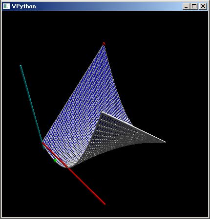
If you come across unkown codes, you can examint them by using np.info(..), np.source(..). If you don't understand the feature of klsp(..), please examine it by np.info(..) and np.source(..). It is easy to examine them using PythonSf one-liners as below.
PythonSf one-liners
# source of klsp(..): just only re-cast a Numpy instance that linspace created to the ClTensor instance.
np.source(klsp)
In file: pysf\basicFnctns.py

def klsp(*sq, **dct):
    """' return ClTensor of scipy.linspace(...)
    '"""
    return sf.krry(sc.linspace(*sq, **dct) )

===============================
None

# ClTensor 50 points data that was created by cutting into equal 49 parts of [-1,1] area
klsp(-1,1)
===============================
[-1.         -0.95918367 -0.91836735 -0.87755102 -0.83673469 -0.79591837
 -0.75510204 -0.71428571 -0.67346939 -0.63265306 -0.59183673 -0.55102041
 -0.51020408 -0.46938776 -0.42857143 -0.3877551  -0.34693878 -0.30612245
 -0.26530612 -0.2244898  -0.18367347 -0.14285714 -0.10204082 -0.06122449
 -0.02040816  0.02040816  0.06122449  0.10204082  0.14285714  0.18367347
  0.2244898   0.26530612  0.30612245  0.34693878  0.3877551   0.42857143
  0.46938776  0.51020408  0.55102041  0.59183673  0.63265306  0.67346939
  0.71428571  0.75510204  0.79591837  0.83673469  0.87755102  0.91836735
  0.95918367  1.        ]
---- ClTensor ----

# ClTensor 6 points data that was created by cutting into equal 5 parts of [-1,1] area
klsp(-1,1, 6)
===============================
[-1.  -0.6 -0.2  0.2  0.6  1. ]
---- ClTensor ----
It is effective not only at PythonSf expressions but alsot at general Python codes to examine Pythonobjects usint np.inf(..), np.source(..). Plese utilize them.
PythonSf primarily uses ClTensor or ClFldTns instances than numpy.ndarray. Because they are easier to calculate vectors or matrices. PythonSf uses ClTensor instances whose elements are integer, float or complex and ClFldTns instances whose elements are not integer, float and complex. Instances which are made by ~[...] expressions are eather ClTensor instances or ClFldTns instances
We list up below why we avoid numpy.ndarray
You would be embarrassed, if you use numpy.ndarray. Because you would unconsciously use makes integer type vectors or matrices for float ones, They would work plausibly and you would accumulate considerations without noticing them. It is difficult to find out erroneous expressions afterward. It is rare in mathematics to distinguish integer and float, because both of them are number. Even though you would be careful for the miss-uses, they would steal into your expressions because of mathematical habits. So ClTensor class makes float type vectors or matrices, if you designate "int" explicitly, although it inherits numpy.ndarray.
We also have implementd functions corresponding to four operations and exponentiation like as __mul__(..), __pow__(..) and others. So you can write expressions of vector, matrices that are more resembled to daily memo writing expressions.
You can calculate four operations between a ClTensor instance and Python sequence as tuple, list, numpy.ndarray, if their dimension is conformed. So you can calculate multiplications between a matrix and vector or inner products between vector and sequence, without using a row vector or column vector as in Matlab. You can look at the examples below.
PythonSf one-liners
# inner product
vc=~[1,2,3]; vc ~[4,5,6]
===============================
32.0

# a inner product between a vector and list
vc=~[1,2,3]; vc  [4,5,6]
===============================
32.0

~[k for k in range(1,4)] [4,5,6]
===============================
32.0

vc=~[1,2,3]; vc range(4,7)
===============================
32.0

# inner product between a vector and tuple
vc=~[1,2,3]; vc  (4,5,6)

# multiplication between a matrix and vector
mt = ~[[1,2],[3,4]]; mt ~[5,6]
===============================
[ 17.  39.]
---- ClTensor ----

# multiplication between a matrix and list
mt = ~[[1,2],[3,4]]; mt  [5,6]
===============================
[ 17.  39.]
---- ClTensor ----

# multiplication between a list and matrix
mt = ~[[1,2],[3,4]]; [5,6] mt
===============================
[ 23.  34.]
---- ClTensor ----

# multiplication between a matrix and tuple
mt = ~[[1,2],[3,4]]; mt  (5,6)
===============================
[ 17.  39.]
---- ClTensor ----
Numpy package has sub packages for random functions, FFT, linear algebra and others these are used frequently, though they are smaller than that of SciPy package. PythonSf utilize them in a positive manner, because it is faster to import numpy than importing scipy.
You can call them like as "np.random.rand(..)". But the calling string are too long for frequent usage. So we implement global buffer functions of these numpy sub packages. In passing we modified them to make return a ClTensor instance: not a numpy.ndarray instance.
The numpy.random module provides functions of radint(..) that returns random integers from the discrete uniform distribution, rand(..) that returns random values between 0 and 1 in a given shape:, randn(..) that returns a sample (or samples) from the standard normal distribution and shuffle(..) that return a modified sequence in-place by shuffling its contents. These functions are very convenient because they can deal with a matrix or vector.
We have implemented rand(..) function as below.
np.source(rand)
In file: pysf\kNumeric.py

def rand(*sqAg):
    if len(sqAg) == 0:
        return        (sf.sc.random.rand(*sqAg))
    else:
        return sf.krry(sf.sc.random.rand(*sqAg))

===============================
None
We have also exchanged functions of seed(..), randint, randn(..) and suffle(..). So you can shortly write expressions that utilize functions in NumPy random package as below.
PythonSf one-liners
# return a randome value in [0,1] range.
seed(0); rand()
===============================
0.548813503927

# return a matrix of that elements are random values in [0,1] range.
seed(0); rand(2,4)
===============================
[[ 0.5488135   0.71518937  0.60276338  0.54488318]
 [ 0.4236548   0.64589411  0.43758721  0.891773  ]]
---- ClTensor ----

# return a matrix of that elements are in the normal distribution
seed(0); randn(2,4)
===============================
[[ 1.76405235  0.40015721  0.97873798  2.2408932 ]
 [ 1.86755799 -0.97727788  0.95008842 -0.15135721]]
---- ClTensor ----

# return a integer type matrix of that elements are integers betwee 0 and 8
randint(9,size=[2,5])
===============================
[[5 6 7 3 1]
 [8 1 1 7 4]]
---- ClTensor ----

# return a floating type matrix of that elements are betwee 0 and 8
~[randint(9,size=[2,5])]
===============================
[[ 1.  0.  5.  2.  4.]
 [ 5.  1.  8.  5.  6.]]
---- ClTensor ----

# return a type matrix of that elements are BF:Bool Field
~[randint(2,size=[2,5]), oc.BF]
===============================
[[0 1 0 0 1]
 [1 1 0 0 0]]
---- ClFldTns:< class 'pysf.octn.BF'> ----
You can verify a formula:sin(2θ)==2sin(θ)cos(θ) by numerical experiment as below.
PythonSf one-liners
# proof/confirm the formulat:sin(2θ)== 2sin(θ)cos(θ)
vc=randn(10); [sin(2θ) for θ in vc] ~== [2 sin(θ) cos(θ) for θ in vc]
===============================
True

# also proof/confirma in complex numbers
# 複素数値でも sin(2θ)== 2sin(θ)cos(θ)
mt=randn(2,10);vc=mt[0,:]+`i mt[1,:];  [sin(2θ) for θ in vc] ~== [2 sin(θ) cos(θ) for θ in vc]
===============================
True
To execute the uuper one-liner means you have confirmed ten times that sin(2θ) is same with 2sin(θ)cos(θ) in 6 digits precision for random θ. "~==" is a user defining infix operator and we have assigned nearlyEq(..) function to it in customize.py file. This function returns true if the arguments are same in more than 6 digits precision. (You can't use "==" operator, because computers use floating numbers and there are accidental errors in calculated results so that formulas is not true for "==" operator. It may be no exaggeration to say that we have proved the formula "sin(2θ)==2sin(θcons(θ)" after confirming 10 times in 6 digits precision. Because errors might sneak into the proof with very higher provability.
You can conveniently use random functions for proofs like this.
There is a function:shuffle(..) in numpy.random module and it permutates elments of a sequence. However the shuffle function returns None. It updates just contents of a reffed argument. But it is strongly required for one-liners to return the reference too. So we modified the shuffle function as below.
PythonSf one-liner
np.source(shuffle)
In file: pysf\kNumeric.py

def shuffle(sqAg):
    sf.sc.random.shuffle(sqAg)
    return sqAg

===============================
None
So you can use it as blow.
PythonSf one-liners
shuffle(range(10))
===============================
[1, 7, 4, 9, 0, 2, 5, 3, 6, 8]

# comparing: shuffle(..) of NumPy
np.random.shuffle(range(10))
===============================
None

lst=range(10); np.random.shuffle(lst); lst
===============================
[6, 8, 0, 3, 1, 5, 9, 4, 7, 2]
(Inverse) Fourier Transform is used frequently in many field. So we should put them in PythonSf global name space. And it is convenient to return a ClTensor instance. So we have modified fft,ifft and fftshift in numpy.fft package.
Note that fft and ifft in NumPy don't conserve a norm. It maintais spectrum density as Matlab. But we strongly require the FFT that maintains norm in mathematics. So we have implemented nft(..) and inft(..)
In addition the FFT deals with arbitrary length sequence. Doesn't limit it's length to 2^N.
We show examples below.
PythonSf one-liners
N=7; fft(range(N))
===============================
[ 21.0+0.j          -3.5+7.26782489j  -3.5+2.79115686j  -3.5+0.79885216j
  -3.5-0.79885216j  -3.5-2.79115686j  -3.5-7.26782489j]
---- ClTensor ----

N=7; ifft(fft(range(N)))
===============================
[  2.91830052e-15+0.j   1.00000000e+00+0.j   2.00000000e+00+0.j
   3.00000000e+00+0.j   4.00000000e+00+0.j   5.00000000e+00+0.j
   6.00000000e+00+0.j]
---- ClTensor ----

N=7; nft(range(N))
===============================
[ 7.93725393+0.j         -1.32287566+2.7469796j  -1.32287566+1.05495813j
 -1.32287566+0.30193774j -1.32287566-0.30193774j -1.32287566-1.05495813j
 -1.32287566-2.7469796j ]
---- ClTensor ----

N=7; inft(nft(range(N)))
===============================
[  2.85344905e-15+0.j   1.00000000e+00+0.j   2.00000000e+00+0.j
   3.00000000e+00+0.j   4.00000000e+00+0.j   5.00000000e+00+0.j
   6.00000000e+00+0.j]
---- ClTensor ----

N=7; norm(fft(range(N))) ~== ( sqrt(N) norm(nft(range(N))))
===============================
True
We have modified matrix functions:expm(.), logm(.) sqrtm(.), egvals(.)/eigvalsh(.) and eig(.)/eigh(.). So they return a ClTensor instance as blow.
PythonSf one-liners
t=0.1; expm(`σx t)
===============================
[[ 1.00500417  0.10016675]
 [ 0.10016675  1.00500417]]
---- ClTensor ----

t=0.1; logm( expm(`σx t) )
===============================
[[ -9.02056208e-17   1.00000000e-01]
 [  1.00000000e-01  -9.02056208e-17]]
---- ClTensor ----

t=0.1; sqrtm(`σx t)
===============================
[[ 0.15811388+0.15811388j  0.15811388-0.15811388j]
 [ 0.15811388-0.15811388j  0.15811388+0.15811388j]]
---- ClTensor ----

t=0.1; sqrtm(`σx t)^2
===============================
[[ 0.0+0.j  0.1+0.j]
 [ 0.1+0.j  0.0+0.j]]
---- ClTensor ----

t=0.1; eigvalsh(`σx t)
===============================
[-0.1  0.1]
---- ClTensor ----

t=0.1; eigh(`σx t)
===============================
(ClTensor([-0.1,  0.1]),
ClTensor([[-0.70710678,  0.70710678],
          [ 0.70710678,  0.70710678]]))

t=0.1; mt=`σx t; mt[1,1]=3; eigvals(mt)
===============================
[-0.00332964  3.00332964]
---- ClTensor ----

t=0.1; mt=`σx t; mt[1,1]=3; eig(mt)
===============================
(ClTensor([-0.00332964,  3.00332964]),
ClTensor([[-0.99944614, -0.03327794],
          [ 0.03327794, -0.99944614]]))
If you have SciPy functions that are not ufunc, you can customize them to return a ClTensor instance like as upper exmaples for short one-liner expressions.
By the way, we have implemented pp(.) function to print just only a vector or matrix for easy-to-understand calculated results by suppressing extra zeros as below.
PythonSf ワンライナー
t=0.1; pp(sqrtm(`σx t)^2)
[[   0, 0.1]
,[ 0.1,   0]]
-------- pp --
===============================
None
SymPy package enable you to deal with symbolic expressions. SymPy is newly developed and is pale before Mathematica,Maxima and others. You might come across a bug, if you write hundreds of SymPy codes. But SymPy is developed to a sufficiently practical level for one-liners.
You must call ts() function to utilize SymPy at a PythonSf one-liner. The function call executes "import sympy as ts" and assign symbolic variables to `x,`y,`z and `t. So you can manipulate symbolic expressions as below.
PythonSf one-liners
# solve below equations for x,y variable
# x+y+z = 6
# x-y   = 0
ts(); ts.solve( [`x+`y+`z-6, `x-`y], [`x,`y] )
===============================
{x: -z/2 + 3, y: -z/2 + 3}

# solve below equations for x,y variable
# (x+z) y = 6
# x-y     = 0
ts(); ts.solve( [(`x+`z) `y-6, `x-`y], [`x,`y] )
===============================
[(-z/2 + (z**2 + 24)**(1/2)/2, -z/2 + (z**2 + 24)**(1/2)/2),
 (-z/2 - (z**2 + 24)**(1/2)/2, -z/2 - (z**2 + 24)**(1/2)/2)]
You can calculte numbers with SI units in PythonSf. We utilize units of sympy.physics.unit. We have assigned units to A`,Ω`,V` and others in customize.py utilizing the extension of name space by "`". You can use them after calling "ts()", because we use SymPy. We show some examples below.
PythonSf ワンライナー
# Voltage/Current--> Resistance
ts(); V,I=3.0V`, 2  A`; V/I
===============================
1.5*V`/A`

# Voltage/Resistance--> Current
ts(); V,R=3.0V`, 1.5Ω`; V/R
===============================
2.0*A`
We have assigned units to f` p` n` u` mili` k` M` G` hour` min` s` ms` us` ns` ps` kg` g` =1, nm` um` mm` cm` m` met met km` inch` feet` mile` C` A` mA` uA` V` mV` uH` F` uF` pF` Ω` kΩ` ohm` Hz` N` J` mLght` in customize.py. You can any hopeful units by adding Python codes at this place.
We have assigned below principal physical constants with units in customize.py.
Python codes
    #=========== physical constants begin ========================
    # light velosity m/s
    k_c_bq____ = 2.99792458e+8 * ut.m / ut.s            #@:c` --> k__bq__c___

    # planck constant h/2π 1.054571628(53)×10-34 J s
    k_h_bq__bq____ = 1.054571628e-34 * ut.J * ut.s      #@:h`` --> h/(2π)
    k_h_bq____ = 6.62606896e-034 * ut.J * ut.s          #@:h` -->


    #Boltzman constant   J K^-1。 K is a unit of absolute temparature. Joule/Kelvin
    k_kB_bq____ = 1.380662e-23 * ut.J / ut.K            #@:kB` -->

    #universal constant of gravitation gU` = 6.67259 ×10⁻¹¹  N` m`^2 `kg-2
    k_gU_bq____ = 6.67259e-11 * ut.N * ut.m**2 / ut.kg**2 #@:gU` -->
    #gravitational constant gH`  = 9.80665  m s-2
    k_gH_bq____ = 9.80665 * ut.m / ut.s**2              #@:gH` -->

    #elementary charge eQ`  = 1.6021892 ×10⁻¹⁹  C
    k_eQ_bq____ = 1.6021892e-19 * ut.C
    #mass of electron eM`  = 9.10938188 ×10^-31  kg
    k_eM_bq____ = 9.10938188e-31 * ut.kg
    #mass of proton pM`  = 1.67262157 ×10^-27  kg
    k_pM_bq____ = 1.67262157e-27 * ut.kg
    #mass of hydrogen atom HM` = 1.6735 ×10^-27  kg
    k_HM_bq____ = 1.6735e-27 * ut.kg
    #number of moles,Avogadro number  NA`  = 6.02214199 ×10^23  mol-1
    k_NA_bq____ = 6.02214199e+23 / ut.mol
    #molal volume Vm`  = 2.241383 ×10⁻²  m3mol-1
    k_Vm_bq____ = 2.241383e-2 * ut.m**3 / ut.mol

    #permeability of vacuume 1.2566370614E-06 == 4`π 1e-7, physical unit N` A`^-2 == henry/meter == weber/(ampere meter)
    k__sMu_0_bq____ = 1.2566370614e-6 * ut.H/ut.m        #@μ0` -->
    k_u0_bq____ = 1.2566370614e-6 *ut.H/ut.m
    # permittivity of vacuum ε0 == 1/(`c^2 4`π 1e-7)==coulomb**2 / (newton * M ** 2) == farad/meter == coulomb/(volt meter)
    k__sEpsilon_0_bq____ = 8.854187816e-12 * ut.F/ut.m  #@:ε0` -->
    k_e0_bq____ = 8.854187816e-12 * ut.F/ut.m

    #=========== physical constants end = ==================================
So you can calculate one-liners as below.
PythonSf one-liner
# E == m c^2 == h ν
# ∴ ν== m c^2/h
# frequency of electron at 4 dimensional space time
ts(); eM` c`^2/h`
===============================
1.23558993864461e+20/s`
What units or physical constants are needed dipends largely on your area of specialization. The units and physical constants of Pythonsf are defined by Python codes in customize.py. You can customize the units and physical constants as you want by modifying the Python codes.
It is convenient and needed to use units consisted of a just only number.
PythonSf expressions with units is explanatory. "15V` * 1.3A`" means a multiplication of a value of voltage and a value of current. So you can guess it will result wattage from just only the PythonSf expression without any other documents.
Arguments with SymPy units is called only by SymPy functions and PythonSf basic numeric functions and four operations, exponentiation and composition of them. General Python functions as in NumPy can't deal with the value of SymPy units, although the SymPy unit's value become the null unit dimension eliminating each other. They will return error comments as below.
PythonSf one-liners
# set a value with SymPy units to NumPy sin function.
ts(); np.sin( 2pi 50Hz` 0.1s`)
Traceback (most recent call last):
    sniped
AttributeError: sin

# set a value with SymPy units to PythonSf basic numeric sin function
ts();    sin( 2pi 50Hz` 0.1s`)
===============================
2.32806687965e-15
It is impossible to set a parameter with units in physics that describe natural law. So PythonSf basic numeric functions except for sqrt(..) and absF(..) will return error comments, if you give a parameter that is not the null dimension eliminating the unit(s) each other.
PythonSf one-liners
# set a parameter with a SymPy unit to PythonSf basic numeric function:sin(..)
ts();    sin( 2pi 50Hz`      )
Traceback (most recent call last):
  File "C:\Python27\lib\runpy.py", line 162, in _run_module_as_main
    "__main__", fname, loader, pkg_name)
  File "C:\Python27\lib\runpy.py", line 72, in _run_code
    exec code in run_globals
  File "D:\my\vc7\mtCm\sfPP.py", line 2, in
    pysf.sfPPrcssr.start()
  File "pysf\sfPPrcssr.py", line 2776, in start
    __execLine( (" ".join(sys.argv[1:])).strip() )
  File "pysf\sfPPrcssr.py", line 2392, in __execLine
    valStt = eval(ustConvertedAt, globals(), locals() )
  File "", line 1, in
  File "pysf\basicFnctns.py", line 854, in __call__
    return self.m_fn(lstGlbAt['Float'](agAt))
  File "pysf\customize.py", line 750, in Float
    + str(fnAt)
AssertionError: At Float(.), you set physical quantity parameter,the units of which are not cancelled:314.159265358979/s`

ts();    sqrt( 2pi 50Hz`      )
===============================
17.7245385090552/s`**(1/2)

ts();    absF(-2pi 50Hz`      )
===============================
314.159265358979/s`
But in engennering there are many functions with parameter(s) that have units. For an example, characteristics of filters can be describe ty funcsions exp(..) and others.
On the other hands, there are no needs to assign SymPy units as Hz`, if you want just only explanatory expressions. As you many assign just number 1 to Hz`, s` and others, the PythonSf expressions are explanatory. So we have decided to assign just number 1 for units before ts() function is called. Then we can use explanatory PythonSf expressions for arbitrary Python functions. We can calculate as below.
PythonSf one-liner
      np.sin( 2pi 50Hz` 0.1s`)
===============================
2.32806687965e-15
Looking at upper, we implemented ts() function. Plese read the souce codes of ts() in pysf\customize.py file, if you are interested in this function.
The written standart of SI unit systemexplains just only how to use it without reasons. And SI is established by compromise to historical backgrounds.backgrounds. Although most engineers regards A:current and V:voltage or ohm:resistance as base units, SI have decided only A:current as a base unit. So that voltage and resistance value is expressed by a combination of M K S A four basic units. Actually sympy.physics.units implements unit system according to SI standard and calculates a expression with units as below.
PythonSf one-liners
# resistance * current:R I == voltage:V
import sympy.physics.units as ut; R,I=1.5ut.ohm, 2ut.A; R I
===============================
3.0*m**2*kg/(A*s**3)

# voltage / current:V/I == resistance:ohm
import sympy.physics.units as ut; V,I=3.0ut.V  , 2ut.A; V/I
===============================
1.5*m**2*kg/(A**2*s**3)

# fine structure constant 1
ts(); eQ`^2/(4pi ε0` h`` c`)
===============================
0.00729746834685501*A`*s`**3*V`/(kg`*m`**2)

# fine structure constant 2
ts(); eQ`^2/(4pi ε0` h`` c`) J`/s`/W`
===============================
0.00729746834685501
But most engineers can't understance the voltage unit:"m**2*kg/(A*s**3)" and the resistance unit:"m**2*kg/(A**2*s**3)". Because they have recognized A:current and V:voltage as base units. でも電圧の単位が「m**2*kg/(A*s**3)」と、また抵抗の単位が「m**2*kg/(A**2*s**3). So the practical unit system should be implemented as MKSAV unit system, not as MKSA unit system. PythonSf have implemented the unit system as MKSAV. You can calculte them as below.
PythonSf one-liners
# resistance * current:R I == voltage:V
ts(); R,I=1.5Ω`, 2A`; R I
===============================
3.0*V`

# voltage / current:V/I == resistance:ohm: V/A
ts(); V,I=3.0V` , 2A`; V/I
===============================
1.5*V`/A`
Do you agree with the claim of MKSAV unit system? Anyway the implementation of unit system is not worth if it is not implemented like as upper expressions.
However, please note that MKSAV unit system is redundant and you should convert the value by multiplying integer power of W` s`/J` by themselves. You should select mechanical, electro-magenetic, ampere, voltage units. Although it is bit bother, it is the unit system that most of engineers appreciate.
We show expressions in MKSAV unit system as below.
PythonSf one-liners
# voltage * current:V I == wattage:W`: A V
ts(); V,I=3.0V` , 2A`; V I
===============================
6.0*A`*V`

# voltage * current:V I == works per a unit time:J`/s`
ts(); V,I=3.0V` , 2A`; V I J`/(W` s`)
===============================
6.0*m`**2*kg`/s`**3

# Force per a unit meter that works between electric wires which saparate 1m --- 1
ts(); u0` A`^2/(2pi m`)
===============================
1.99999999994284e-7*A`*s`*V`/m`**2

# Force per a unit meter that works between electric wires which saparate 1m --- 2
ts(); u0` A`^2/(2pi m`) J`/s`/W`
===============================
1.99999999994284e-7*kg`/s`**2

# Force that works between chages which saparate 1m --- 1
ts(); 1.0C`^2/(4pi e0` 1m`^2)
===============================
8987551789.01297*A`*s`*V`/m`
# Force that works between chages which saparate 1m --- 2
ts(); 1.0C`^2/(4pi e0` 1m`^2) J`/s`/W`
===============================
8987551789.01297*kg`*m`/s`**2

# Electric Field made by charges which separate 1m
ts(); 1.0C`/(4pi e0` 1m`^2)
===============================
8987551789.01297*V`/m`

# Electric Potential made by charges which separate 1m
ts(); 1.0C`/(4pi e0` 1m`)
===============================
8987551789.01297*V`

# Magnetic Flux:Φ made by a 1uH coil with 1A current
ts(); 1.0uH` 1A`
===============================
1.0e-6*s`*V`

# Fine Structure Constant 1
ts(); eQ`^2/(4pi ε0` h`` c`)
===============================
0.00729746834685501*A`*s`**3*V`/(kg`*m`**2)

# Fine Structure Constant 2
ts(); eQ`^2/(4pi ε0` h`` c`) J`/s`/W`
===============================
0.00729746834685501
You can see same sexpression in sympy.physics.units:MKSA unit system as below.
PythonSf one-liners
# voltage * current:V I == wattage
import sympy.physics.units as ut; 3.0 ut.V 2ut.A
===============================
6.0*kg*m**2/s**3

# Force per a unit meter that works between electric wires which saparate 1m
import sympy.physics.units as ut; ut.u0 1.0ut.A^2/(2pi ut.m)
===============================
6.36619772367581e-8*pi*kg/s**2

# Electric Field made by charges which separate 1m
ts(); import sympy.physics.units as ut; 1.0ut.C/(4pi ut.e0 1ut.m^2) 3.14159265359/ts.pi
===============================
8987551787.36877*kg*m/(A*s**3)

# Electric Potential made by charges which separate 1m
ts(); import sympy.physics.units as ut; 1.0ut.C^2/(4pi ut.e0 1ut.m^2) 3.14159265359/ts.pi
===============================
8987551787.36877*kg*m/s**2

# Magnetic Flux:Φ made by a 1uH coil with 1A current
import sympy.physics.units as ut; 1e-6 ut.H ut.A
===============================
1.0e-6*kg*m**2/(A*s**2)

# Fine Structure Constant
ts(); import sympy.physics.units as ut; eQ,h,c=1.6021892e-19 ut.A ut.s, 1.054571628e-34 ut.kg ut.m^2/ut.s, 299792458.0ut.m/ut.s; eQ^2/(4.0 pi ut.e0 h c) 3.14159265359/ts.pi
===============================
0.00729746834552000
At Fine Structure Constant, SI:MKSA unit system is more convenient, But it is not worth, because the units of electric field or potential are kg*m/(A*s**3) or kg*m/s**2. Engineers can't understand them, although they frequently deal with them.
But PythonSf:MKSAV unit system shows Electric Field/Potenial units with V`/m` ro V`. Engineers can use MKSAV unit system practically. They use MKSAV units.
In python, there are paccages showing graphs such as pylab, mayavi. They are great ones that can draw high quality graphs that can be used in research papers.
But they are too bother to draw graphs. There are no needs of explanatory notes for graphs drawn for yourself, because you have known them. You might not need a scale of a horizontal axis. You needs ways to draw graphs with least pains, because you might want to see the graphs without a moment's delay. So PythonSf have implemented drawing functions: plotGr(..), plotTrajectory(..), plot3dGr(..), renderFaces(..), plotTmCh(..).
PythonSf one-liner
plotGr(sin( 2pi `X^2)  )
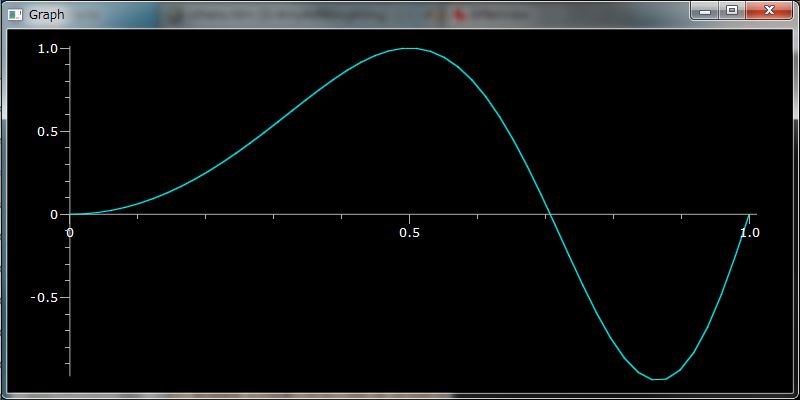
If you want a graph drawn on a interval:[-2,3] at 256 points data, you should set parameters to PlotGr(..) as below.
PythonSf one-liner
plotGr(sin( 2pi `X^2), -2, 3, 256)
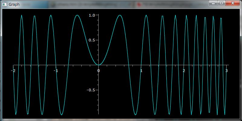
You can draw a graph with sequence data such as tuple, list, array and others. Please note that the horizontal scale is len(sequnce date). But there is no problems because you look at the graph that is drawned by yourself withe the one-liner:"plotGr([sin( 2pi `X^2)(t) for t in klsp(-2,2, 128)])", and you know the horizontal intarbal is [-2,2].
PythonSf one-liner
plotGr([sin( 2pi `X^2)(t) for t in klsp(-2,2, 128)])
If you set plotTrajectory(..) a 2 dimensional position sequence data, it draws a 2 dimensional graph that connects the positions with lines as below.
PythonSf one-liner
plotTrajectory([(0.9 cos(θ),sin(2θ)) for θ in arsq(0, 256,2pi/256)])
If you set plotTrajectory(..) a 3 dimensional position sequence data, it draws a 3 dimensional graph.
PythonSf one-liner
plotTrajectory([(0.9 cos(θ),sin(2θ), θ) for θ in arsq(0, 256,2pi/256)])
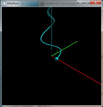
If you want to study a 3 dimensional shapes of 2 variables function:f(x,y), you should use plot3DGr(..).
PythonSf ワンライナー
plot3dGr(sin(`X) cos(`Y), [-pi,pi],[pi,-pi])
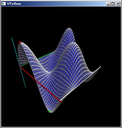
plot3dGr(..) can render a 4 dimensional shape of a complex value function on complex plain. The shape consists of hight of the complex value and the phase which is rendered as mixed colors of red,green and blue.
PythonSf ワンライナー
plot3dGr(sin(`X) cos(`X), [-pi,pi],[pi `i,-pi `i])
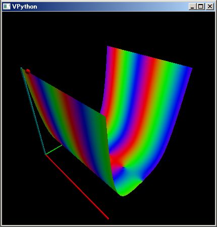
PythonSf ワンライナー
plot3dGr(log, [-pi,pi],[pi `i,-pi `i])
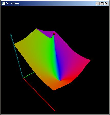
You might often want to visualize a distribution in a rectangular arear. Because it is difficult to grasp tendencies just from a bunch of data. You can grasp the tendencies at a glance from 3d visualized graphs
PythonSf one-liners


seed(0);vc=~[range(10)]; renderMtrx(vc^vc + 3 randn(10,10))
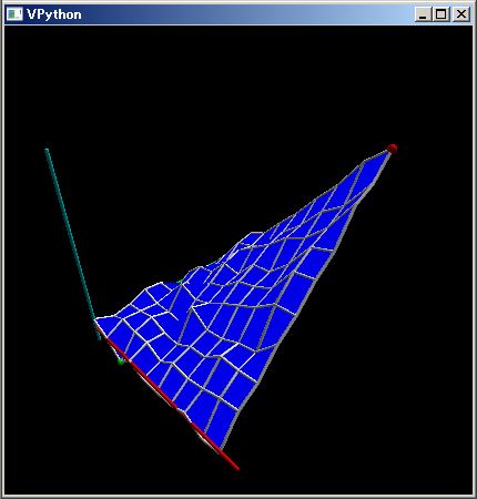
You can render a distribution of complex values in a mtraix as a 3d graph where the phase rotations are drawn by mixing rate of RGB colors.
PythonSf one-liner


seed(0); vc=~[range(10)]; renderMtCplx(vc^vc+3(randn(10,10)+`i randn(10,10)))
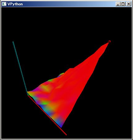
You can render a 3 dimentional curved surface by setting renderFaces(.) a matrix parameter where the elements are 3 dimensional position vectors. We show a example below.
PythonSf one-liner


# Moebius strip

dct={}; for idx, (u,v) in enmitr(klsp(0,2pi),klsp(-1,1,10)):dct[idx]=((1+0.5v cos(0.5u))cos(u), (1+0.5v cos(0.5u))sin(u), 0.5v sin(0.5u)); renderFaces(dct,blMesh = True)
It is convinient to use a dictionary for a matrix where the elements are position vector as the upper example code. Because you don't neet to declare a matrix consistent with element's type. You don't need to think a matrix where elements are position vectors.
PythonSf one-liner
# Klein bottle
//@@
dct,N,M,r={},64,32,5;
for (u,v), index in zip(masq([0,N,2pi/N], [-1,M+1,2pi/M]), mrng(N,M+1) ):
    dct[index]=( (r+cos(u/2) sin(v)-sin(u/2) sin(2v)) cos(u)
                ,(r+cos(u/2) sin(v)-sin(u/2) sin(2v)) sin(u)
                ,sin(u/2) sin(v) + cos(u/2) sin(2*v) )

sf.renderFaces(dct, blMesh = True)
sf.drawAxis()
//@@@
You can render a 3 dimentional colored curved surface, if you set renderFacesWithRGG(.) a parameter dictionary matrix where elements are pairs of a position vector and a RGB color value. We show a example below.
PythonSf one-liner
# Spherical harmonics

m,l=0,2;sy();clAt = ClCplxColor();psCl=λ θ,φ:(λ cplxAg=ss.sph_harm(m,l,φ,θ):(abs(cplxAg) ~[sin(θ)cos(φ),sin(θ)sin(φ),cos(θ)], clAt.GetFltColor(0.99 cplxAg/abs(cplxAg))))();dct={};for idx,(θ,φ) in enmitr(klsp(0,pi),klsp(0,2pi)):dct[idx]=psCl(θ,φ);renderFacesWithRGB(dct)
We have implemented render2dRGB(..) that renders a complex value distribution in a matrix for a complex value function by a way named as kkRGB.
You shold set parameters as below np.info(render2dRGB). mtrAg is a complex value matrix. it buid up a rectangular jpg picture of which each pixels are corresponding to each complex value elements of the matrix. The phase angles of the complex ue elements correspond to the mixing rate of RGB colors. And the absolute values of them correspond the brightness of the pixels. If you set a 100x100 matrix then it renders a small 100x100 pixcel picture.
PythonSf one-liner
np.info(render2dRGB)
 render2dRGB(mtrxAg, boundary=1.0, limit=10.0, blReverse=False, blBoth=False,
             fileName='kkRGB', blDisplay=True, blMax=False)

' Render a complex value distribution with kkRGB color for matrix argument
        rendered figure is saved at kkRGB.jpg file as a default
    e.g.
vc=klsp(-3,3,300); f=`X^3+`X^2+`X+1; dct={};for idx,(x,y) in enmitr(vc,vc):dct[idx]=f(x+`i y); render2dRGB(dct)
    '
===============================
None
Let render a complex value distribution of a polynomial:`X^3+`X^2+`X+1 by render2dRGB(..) function as below. (render2dRGB(..) function creates kkRGB.jpg file in the current directory using Python Image module and execute the jpg file with start command. In other words, the jpg file is shown by a default program that is associated to the extension name at Windows OS)
PythonSf one-liner


vc=klsp(-3,3,300); f=`X^3+`X^2+`X+1; dct={};for idx,(x,y) in enmitr(vc,vc):dct[idx]=f(x+`i y); render2dRGB(dct)
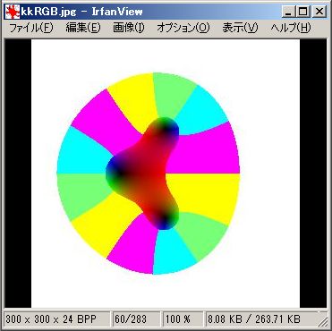
The centers of the three faded black dots in the upper view correspond to positions of complex roots in x^3+x^2+x+1 polynomial. Values of the function is 0 at the roots, so their brightness is 0. You can get the roots by below PythonSf expressions. 上の図で中央に分布している三つのぼやけた黒い丸い領域の中心が、多項式 x^3+x^2+x+1 の複素根の位置に対応しています。根の位置で関数値が 0 になるので、その明度も 0 になっています。(この多項式の根は、下の PythonSf 式で求められます。)
PythonSf one-liners
poly1d([1,1,1,1],variable='x')
===============================
   3     2
1 x + 1 x + 1 x + 1

poly1d([1,1,1,1]).roots
===============================
[ -1.00000000e+00+0.j  -7.77156117e-16+1.j  -7.77156117e-16-1.j]
The boundary between the four colored area and the center continuously colored center area is a place where absolute value of the function is 1 that are assigned by the default parameter:boundary=1.0.
The boundary between the white area and the four colored areas is a place where absolute value of the function is 10 that is assigned by the default parameter:limit=10.0. These four colors correspond four areas that are separated the real line and the imaginary line. So the boundaries between red areas and yellow areas are the part where values of the function are positive real numbers and the boundaries between yellow areas and green areas are the part where values of the function are positive imaginary numbers. You might be able to understand phase changes more easily by four colored areas than by vague continuous RGB rendering. For example, from the upper kkRGB graphic you can easily look that a contour and iso-phase lines of complex analytic function are orthogonal. (Complex analytic functions have this property generally.)
You can render a complex value distribution of a polynomial x^3+x^2+x+1 by plot3dGr(..) function in short as below. But you might be able to image the complex value distribution by render2dRGB(..) more easily.
PythonSf one-liner


plot3dGr(`X^3+`X^2+`X+1, [-3,3],[3`i,-3`i])
You can render a Mandelbrot set by render2dRGB(..) as below.
PythonSf block


//@@
N=512;
def check(c,z=0,k=0):
    return k>500 and 500 or abs(z) < 2 and check(c,z^2+c,k+1) or k;

dct={};
for idx,(x,y) in enmasq((-2,N,4/N),(2`i,N,-4`i/N)):
    dct[idx]=check(x+y);

def convertTo4cplxVl(inAg):
    return inAg==500 and 0.1+0j or inAg>30 and 1+0j  or inAg>10 and 1j or inAg>5 and -1+0j or -1j

for idx in mrng(N,N):
    dct[idx]=convertTo4cplxVl(dct[idx]);

render2dRGB(dct)
//@@@

You can plot time charts of row data in a matrix by setting plotTmCh(..) the matrix parameter. Let plot a time chart with actions of the below 1 bit D/A converter.
ΔΣ DA converter                   in >= 2**15 --> 1
                                    in <  2**15 --> 0
   16  +┌───┐  +   ┌──┐    ┌────────┐    1
→─/─┤Adder ├─→○┤z^-1├┬─┤Digtal      1bit├┬─/───/\/\/\/─┬────
    ┌─┤      │   -↑└──┘│  │Comparator  D/A ││                          │
    │ -└───┘    └────┘  └────────┘│                        ─┴─
    │                  integrator                      │                        ─┬─ C/s
    └─────────────────────────┘                          │
                                                                                    ┴
             Δ            Σ                                                        =
 A:入力                  B:intergrator:countor             C:output: 1 or -1
The below PythonSf one-liner plots variations over time at A,B,C points in the uuper 1bit D/A convertoer on a time-chart after calculating them.
PythonSf one-liner


N=256;f=λ sg,ds,out:(λ dsAg=ds+sg-out*2^15:[sg,dsAg,1 if dsAg>0 else -1])();mt=kzrs(3,N); mt[:,0]=(0,0,0);for i in range(N-1):mt[:,i+1]=f(2^15 sin(2pi i/N),*mt[:,i][1:]);plotTmCh(mt)
It is easy to implement graph functions by users. Because there are graphic packages like as pylab in Python. The source code of the plotTmCh(..) function is open to public. You can acces to the source code just with a below PythonSf one-liner.
PythonSf ワンライナー
np.source(plotTmCh)
In file: pysf\vsGraph.py

def plotTmCh(vctMtrxAg):
    """' plot time chart for vector,array or matrix dictionary data
    '"""
    import pylab as pb
    def __plotTmChX(vctMtrxAg):
        n = len(vctMtrxAg)
        lstYAt = [None]*(2*n)
        lstYAt[0::2] = vctMtrxAg
        lstYAt[1::2] = vctMtrxAg
        lstYAt = [vctMtrxAg[0]]+lstYAt+[vctMtrxAg[-1]]

        lstXAt = [None]*(2*(n+1))
        lstXAt[0::2] = range(n+1)
        lstXAt[1::2] = range(n+1)

        maxAt = max(vctMtrxAg)
        minAt = min(vctMtrxAg)
        pb.plot(lstXAt, lstYAt)

        if maxAt != minAt:
            lstAxisAt = list(pb.axis())
            meanAt = float(maxAt + minAt)/2
            lstAxisAt[2] = minAt + (minAt - meanAt)*0.2 # set Y axis min
            lstAxisAt[3] = maxAt + (maxAt - meanAt)*0.2 # set Y axis max
            pb.axis(lstAxisAt)

    assert '__getitem__' in dir(vctMtrxAg)
    if isinstance(vctMtrxAg, dict) or '__len__' in dir(vctMtrxAg[0]):
        if isinstance(vctMtrxAg, list):
            assert not('__getitem__' in dir(vctMtrxAg[0][0]))
            colSizeAt = len(vctMtrxAg)
        elif isinstance(vctMtrxAg, dict):
            lstAt = vctMtrxAg.keys()
            lstAt.sort()
            shapeAt = lstAt[-1]
            shapeAt = (shapeAt[0]+1, shapeAt[1]+1)
            assert shapeAt[0]*shapeAt[1] == len(lstAt),\
                "dictionary vctMtrxAg index is not alined" + str(objarAg)

            krAt = kzrs(shapeAt)
            for index in sf.mrng(*shapeAt):
                krAt[index] = vctMtrxAg[index]

            vctMtrxAg = krAt
            colSizeAt = shapeAt[0]
        else:
            assert isinstance(vctMtrxAg, sf.sc.ndarray)
            assert len( vctMtrxAg.shape ) == 2

            colSizeAt = vctMtrxAg.shape[0]

        for i, elmAt in enumerate(vctMtrxAg):
            # don't use subplot(,,0) not to shift upper
            pb.subplot(colSizeAt, 1, i+1)
            __plotTmChX(elmAt)
    else:
        __plotTmChX(vctMtrxAg)

    pb.show()

===============================
None
You might guess that it is difficult to implement functions displaying graphs. Using VPython or Matplotlib packages, the graph function in PythonSf are small code size. You can see their codes in one screen. They are open to the public. You can see them with upper the PythonSf one-liner and modify them. There are suited graph functions for each users. Please try to implement your graph functions. You can use them in PythonSf expressions, simply declaring them in sfCrrntin.py or custormize.py file.
scipy.integrate.quad is famous at nemerical integration. But the quad(..) function returns a tuple of an integrated value and the estimated error. On first glance it is good to return an integrated value and the error. But it is bad for one-liner expressions in many cases which process integrated values, because it is necessary to pull out the integrated value from the tuple. So we implemented quadR(..) function that simply returns an integrated value.
Python の数値積分では scipy.integrate.quad が有名です。でも、この quad(..) 関数は、積分値と、その推測誤差の tuple pair を返してくれます。計算誤差まで返してくれるのは、一見良さそうですが、グラフを描かせたりするときは積分値のみを取り出す必要があり、ワンライナーで短く書くには返って不都合です。そのため quadR(..) 関数を実装しています。
また複素数値関数や調和関数の積分も行えるようにしたいので、PythonSf では計算誤差を返さない、積分値のみを返す quadC, quadAn 関数も用意しています。
quadR(実数値関数, 下限、上限) と引数を与えることで数値積分を計算します。下限・上限値には無限大:sy.inf を指定することも可能です。
PythonSf ワンライナーたち
# pi
#∫ sin(x) dx == 2
# 0
quadR(sin, 0,pi)
===============================
2.0

# scipy.integrate quad による積分
sy(); si.quad(sin, 0,pi)
===============================
(2.0, 2.220446049250313e-14)

# ∞ 範囲の積分
# ∞
#∫ exp(-x^2) dx == π^0.5
#-∞
# SciPy の quad(..) であり計算誤差の推定値も含めた計算結果を返す
sy();si.quad(exp(-`X^2), -sy.inf, sy.inf)
===============================
(1.7724538509055159, 1.4202636756658795e-08)

# PythonSf の quadR(..) であり積分値の計算結果のみを返す。誤差は返さない。
quadR(exp(-`X^2), -np.inf, np.inf)
===============================
1.77245385091

# 参考 π^0.5
sqrt(pi)
===============================
1.77245385091

print '%1.20f'%sqrt(pi)
1.77245385090551590000
-------------------------------
None
quadC(複素数値関数, 下限、上限) と引数を与えることで、複素数値関数の数値積分を計算します。
PythonSf ワンライナー
# Fourier Transform function value
~[quadC(exp(2pi `i ν `X) exp(-`X^2), -np.inf, np.inf) for ν in arsq(0,5,1/5)]
===============================
[ 1.77245385+0.j  1.19432452+0.j  0.36539667+0.j  0.05075766+0.j
  0.00320135+0.j]
---- ClTensor ----

# Fourier Transform function of exp(-X^2)
F_f=λ f:( quadC(exp(-2pi `i ν `X) exp(-X^2),-np.inf, np.inf) ).real
Waring: don't use assignment at last sentence.We ignore the assignment.
===============================
 at 0x0213A070>
not picklable

F_f=λ f:( quadC(exp(-2pi `i f `X) exp(-`X^2),-np.inf, np.inf) ).real;F_f(3)
===============================
1.32810429321e-13

# フーリエ変換された関数の実数値分布のグラフ表示
F_f=λ f:( quadC(exp(-2pi `i f `X) exp(-`X^2),-np.inf, np.inf) ).real; plotGr(F_f,-2,2)
quadAn(.)に、quadAn(複素領域を定義域とする関数, [複素数値のリスト]) 被積分関数と直線で結んだ積分経路を与えることで、その積分経路に沿った積分値を計算します。下に例を示します。
PythonSf ワンライナー
quadAn(log, [1,`i,-1,-`i,1])
===============================
((-1.1102230246251565e-16-6.283185307179586j), 3.238303350943406e-09, 3.238303350943406e-09)

quadAn(log, [1,`i,-1,-`i,1])[0] ~== (-2 pi `i)
===============================
True
quadAn(..) のときは、予測される積分計算誤差も実数部、虚数部ともに返しています。
SciPy の integrate パッケージには ode(..) 関数が備わっています。でも時不変な系についても t を明示的に記述せねばならないなど使い方が少しばかり面倒です。ワン・ライナーでは ode(..) を使えません。
そこで kOde(..) 関数を作りました。大部分の場合で kOde(..) の方が使いやすいでしょう。下のように使います。
PythonSf ワンライナー
np.info(kOde)

 kOde(f, x0, t, N=50)

' time independent Runge Kutta integral by scipy.integrate.ode.

kOde(f, x0, t, N=50)
  f:a dynamic equation that may return a vector or list
  x0: a initial codition value that may be a scalar,vector or list
  t: integrating time [0,t]
  N: returning data size

  f doesn't include t term unlike scpy.integrate.ode(..)

  e.g.

  kOde(~[-2 `X `Y, -`X], [1,2], 2s`,10)
  ===============================
  [[  4.63620997e-01   1.86108060e+00]
   [  2.23487176e-01   1.79540724e+00]
   [  1.09764092e-01   1.76345232e+00]
   [  5.44058566e-02   1.74768585e+00]
   [  2.70894588e-02   1.73985328e+00]
   [  1.35187020e-02   1.73594893e+00]
   [  6.75396145e-03   1.73399941e+00]
   [  3.37618618e-03   1.73302515e+00]
   [  1.68817038e-03   1.73253807e+00]
   [  8.44242482e-04   1.73229450e+00]]
  ---- ClTensor ----

        snipped
上の式で ~[-2 `X `Y, -`X] は下の常微分方程式を意味します。
  d  | x |  == |  -2 x y |
 ---(|   |)    |         |
  dt | y |     |  -x     |
`X, `Y は加減乗除べき乗算が可能な恒等関数であり、~[-2,`X `Y, -`X] はベクトル関数です。
PythonSf ワンライナー
~[-2 `X `Y, -`X](2,3)
===============================
[-12.  -2.]
---- ClTensor ----
kOde(..) を使えば、二次元での N 体問題を解くワンライナーを次のように記述できます。D=2 が二次元を意味しています。inV=[....] に設定する初期位置・速度パラメータの数より、粒子数 N が決まります。
getFV(v,i,k) 関数は、位置・速度パラメータ群ベクトル v に対して、 i 番目と k 番目の粒子の間に働く力を求める関数です。(λ r=krry(v[D k:D (k+1)])-krry(v[D i:D (i+1)]):r/norm(r)^3 if norm(r)!=0 else ~[0,0])() は closure 関数の記述と呼び出しです。i 番目と k 番目の粒子の間の距離 r を定める let 文の役割をデフォルト引数機能使って実装しています。λ 式中では assign 文を使えないので、このようなテクニックを使います。
sumFc(v,j) は、位置・速度パラメータ群ベクトル v に対して、j 番目の粒子に働く力を、 getFV(v,j,k) を足し合わせることで求めています。
粒子数 N 個によって変わる軌跡の色を設定するために、複素数の位相による色指定法:ClCplxColor() を使っています。
PythonSf ワンライナー


D=2;inV=[-0.97m`,0.243, 0.97,-0.243, 0,0, 1,1,  -0.466m`/s`,-0.432, -0.466,-0.432, 0.932,0.864, 0,0]; N=len(inV)//(2D) ; getFV=λ v,i,k:(λ r=krry(v[D k:D (k+1)])-krry(v[D i:D (i+1)]):r/norm(r)^3 if norm(r)!=0 else ~[0,0])(); sumFc=λ v,j:sum([getFV(v,j,k) for k in range(N) if j!=k]); fnc= λ *v: np.r_[v[D N:],(~[sumFc(v,j) for j in range(N)]).r]; mt=kOde(fnc,inV, 2 s`,400); cl=ClCplxColor(); for k in range(N):plotTrajectory(mt[:,D k:D (k+1)],color=cl.GetFltColor(exp(`i 2pi k/N)))
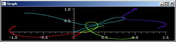
三次元での N 体問題を解くワンライナーは下の様に書けます。
PythonSf ワンライナー


D=3;inV=[-0.97m`,0.243,0, 0.97,-0.243,0, 0,0,1, 1,1,1,  -0.466m`/s`,-0.432,0, -0.466,-0.432,0, 0.932,0.864,0, 0,0,0]; N=len(inV)//(2D) ; getFV=λ v,i,k:(λ r=krry(v[D k:D (k+1)])-krry(v[D i:D (i+1)]):r/norm(r)^3 if norm(r)!=0 else ~[0,0])(); sumFc=λ v,j:sum([getFV(v,j,k) for k in range(N) if j!=k]); fnc= λ *v: np.r_[v[D N:],(~[sumFc(v,j) for j in range(N)]).r]; mt=kOde(fnc,inV, 2 s`,400); cl=ClCplxColor(); for k in range(N):plotTrajectory(mt[:,D k:D (k+1)],color=cl.GetFltColor(exp(`i 2pi k/N)))
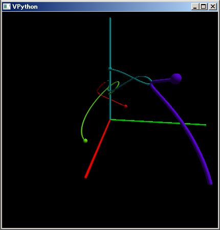
Python Sf における、少し高度な行列演算について説明します。
PythonSf ワンライナー
# ~[ リスト内包表記 ] によるベクトル
~[k^2 for k in range(5)]
===============================
[  0.   1.   4.   9.  16.]
---- ClTensor ----

# ~[ リスト内包表記 ] による行列生成
~[[k j for k in range(5)] for j in range(4)]
===============================
[[  0.   0.   0.   0.   0.]
 [  0.   1.   2.   3.   4.]
 [  0.   2.   4.   6.   8.]
 [  0.   3.   6.   9.  12.]]
---- ClTensor ----

# ~[ リスト内包表記 ] による Zp(5) 要素の行列生成
~[[Z5(k j) for k in range(5)] for j in range(4)]
===============================
[[Z5(0) Z5(0) Z5(0) Z5(0) Z5(0)]
 [Z5(0) Z5(1) Z5(2) Z5(3) Z5(4)]
 [Z5(0) Z5(2) Z5(4) Z5(1) Z5(3)]
 [Z5(0) Z5(3) Z5(1) Z5(4) Z5(2)]]
---- ClFldTns:< class 'sfCrrntIni.Z5'> ----

# ~[ リスト内包表記 ] によって生成された、Zp(5) 要素の行列によるベクトルの変換
~[[Z5(k j) for k in range(5)] for j in range(4)] range(3,3+5)
mt=~[[Z5(k j) for k in range(5)] for j in range(4)]; mt range(3,3+5)
===============================
[Z5(0) Z5(0) Z5(0) Z5(0)]
---- ClFldTns:< class 'sfCrrntIni.Z5'> ----

mt=~[[Z5(k j) for k in range(5)] for j in range(4)]; mt range(2,2+5)
===============================
[Z5(0) Z5(0) Z5(0) Z5(0)]
---- ClFldTns:< class 'sfCrrntIni.Z5'> ----
N x M 行列を越えて、N x M x L などの多次元のテンソルも扱えます。それらとベクトルとの積演算も可能です。次のような具合です。
PythonSf ワンライナー
ls=range(3); ~[ [[x+y+z for x in ls] for y in ls] for z in ls]
===============================
[[[ 0.  1.  2.]
  [ 1.  2.  3.]
  [ 2.  3.  4.]]

 [[ 1.  2.  3.]
  [ 2.  3.  4.]
  [ 3.  4.  5.]]

 [[ 2.  3.  4.]
  [ 3.  4.  5.]
  [ 4.  5.  6.]]]
---- ClTensor ----

PythonSf ワンライナー
# 3x3x3Tensor * 3Vector
ls=range(3); tns=~[ [[x+y+z for x in ls] for y in ls] for z in ls]; tns ls
===============================
[[  5.   8.  11.]
 [  8.  11.  14.]
 [ 11.  14.  17.]]
---- ClTensor ----

PythonSf ワンライナー
# 3Vector * 3x3x3Tensor * 3Vector
ls=range(3); tns=~[ [[x+y+z for x in ls] for y in ls] for z in ls]; ls tns ls
===============================
[ 30.  39.  48.]
---- ClTensor ----

PythonSf ワンライナー
# テンソルどうしの積:Γ`__[j,k,i]  Γ`__[i,p,q]
ls=range(3); Γ`__=~[ [[x+y+z for x in ls] for y in ls] for z in ls]; Γ`__ Γ`__
===============================
[[[[  5.   8.  11.]
   [  8.  11.  14.]
   [ 11.  14.  17.]]

  [[  8.  14.  20.]
   [ 14.  20.  26.]
   [ 20.  26.  32.]]

  [[ 11.  20.  29.]
   [ 20.  29.  38.]
   [ 29.  38.  47.]]]


 [[[  8.  14.  20.]
   [ 14.  20.  26.]
   [ 20.  26.  32.]]

  [[ 11.  20.  29.]
   [ 20.  29.  38.]
   [ 29.  38.  47.]]

  [[ 14.  26.  38.]
   [ 26.  38.  50.]
   [ 38.  50.  62.]]]


 [[[ 11.  20.  29.]
   [ 20.  29.  38.]
   [ 29.  38.  47.]]

  [[ 14.  26.  38.]
   [ 26.  38.  50.]
   [ 38.  50.  62.]]

  [[ 17.  32.  47.]
   [ 32.  47.  62.]
   [ 47.  62.  77.]]]]
---- ClTensor ----

PythonSf ワンライナー
# Einstein 既約による縮約:Γ`__[j,k,k]  Γ`__[m,k,k]
ls=range(3); Γ`__=~[ [[x+y+z for x in ls] for y in ls] for z in ls]; ~[ [sum([Γ`__[j,k,k] Γ`__[m,k,k] for k in ls]) for j in ls] for m in ls]
===============================
[[ 20.  26.  32.]
 [ 26.  35.  44.]
 [ 32.  44.  56.]]
---- ClTensor ----
テンソル演算は手計算では大変すぎて簡単には扱えませんでした。でも PythonSf を使えば、上のようにテンソル演算も簡単であり実用的に使えます。
スカラー値への ^ 演算子の適用はべき乗演算子の意味でしたが、ベクトルや行列の組への ^ 演算子の適用はダイアディック・ベクトル積などのテンソル演算の意味にしています。下のような具合です。
PythonSf ワンライナー ~[1,2,3]^[4,5,6] =============================== [[ 4. 5. 6.] [ 8. 10. 12.] [ 12. 15. 18.]] ---- ClTensor ---- ~[1,2,3]^~[4,5,6]^~[7,8,9] =============================== [[[ 28. 32. 36.] [ 35. 40. 45.] [ 42. 48. 54.]] [[ 56. 64. 72.] [ 70. 80. 90.] [ 84. 96. 108.]] [[ 84. 96. 108.] [ 105. 120. 135.] [ 126. 144. 162.]]] ---- ClTensor ---- `σx ^ `σz =============================== [[[[ 0. 0.] [ 0. -0.]] [[ 1. 0.] [ 0. -1.]]] [[[ 1. 0.] [ 0. -1.]] [[ 0. 0.] [ 0. -0.]]]] ---- ClTensor ----ベクトルの外積演算は Levi-Civita tensor とベクトルとの積によって計算できます。その他にも複数の方法が使えます。
PythonSf ワンライナーたち # Levi-Civita tensor `εL とベクトルとの積演算による外積 a,b=~[1,2,3],~[4,5,6]; -a `εL b =============================== [-3. 6. -3.] ---- ClTensor ---- # Numpy cross 関数による外積 np.cross([1,2,3],[4,5,6]) =============================== [-3 6 -3] # ^ 演算子による外積 a,b=~[1,2,3],~[4,5,6]; a^b - b^a =============================== [[ 0. -3. -6.] [ 3. 0. -3.] [ 6. 3. 0.]] ---- ClTensor ---- # Wedge 積関数 `Λ(..) による外積 a,b=~[1,2,3],~[4,5,6]; `Λ(a,b) =============================== [[ 0. -3. -6.] [ 3. 0. -3.] [ 6. 3. 0.]] ---- ClTensor ----
三次元だけで使うときは np.cross(..) が良いのかもしれません。
私自身は a^b-b^a や `Λ(a,b) による外積演算が優れていると思います。任意の N 次元ベクトルにも使えるからです。計算結果をベクトルではなくテンソルにしておいたほうが、外積の数学的・物理学的な意味が明確になるからです。このときは三次元ベクトルどうしの外積が 3x3 反対称行列になってしまいますが、こちらの方が本来の数学的・物理学的な意味を表しています。
とくに外積の拡張としての Wedge 積関数:`Λ(..) が微分形式に慣れた方に便利だと思います。任意個数、任意次元のベクトルについて Wedge 積を計算できます。ただし行列を引数としたときまでは実装してありません。誤った計算値になります。御注意ください。
PythonSf ワンライナー
a,b=[1,2,3,4],[5,6,7,8]; `Λ(a,b)
===============================
[[  0.  -4.  -8. -12.]
 [  4.   0.  -4.  -8.]
 [  8.   4.   0.  -4.]
 [ 12.   8.   4.   0.]]
---- ClTensor ----

a,b,c=[1,2,3,4],[5,6,7,8],[9,10,11,12]; `Λ(a,b,c)
===============================
[[[ 0.  0.  0.  0.]
  [ 0.  0.  0.  0.]
  [ 0.  0.  0.  0.]
  [ 0.  0.  0.  0.]]

 [[ 0.  0.  0.  0.]
  [ 0.  0.  0.  0.]
  [ 0.  0.  0.  0.]
  [ 0.  0.  0.  0.]]

 [[ 0.  0.  0.  0.]
  [ 0.  0.  0.  0.]
  [ 0.  0.  0.  0.]
  [ 0.  0.  0.  0.]]

 [[ 0.  0.  0.  0.]
  [ 0.  0.  0.  0.]
  [ 0.  0.  0.  0.]
  [ 0.  0.  0.  0.]]]
---- ClTensor ----

# 四次元 Zp(3) ベクトルの外積
a,b=~[1,2,3,4,Z3],~[5,6,7,8,Z3]; `Λ(a,b)
===============================
[[Z3(0) Z3(2) Z3(1) Z3(0)]
 [Z3(1) Z3(0) Z3(2) Z3(1)]
 [Z3(2) Z3(1) Z3(0) Z3(2)]
 [Z3(0) Z3(2) Z3(1) Z3(0)]]
---- ClTensor ----

# 下の Pauli 行列の Wedge 積の計算値は誤りです。行列引数はサポートしていません。
`Λ(`σx,`σz)
===============================
[[[[ 0. -1.]
   [-1.  0.]]

  [[ 1.  0.]
   [ 0. -1.]]]


 [[[ 1.  0.]
   [ 0. -1.]]

  [[ 0.  1.]
   [ 1.  0.]]]]
---- ClTensor ----
PythonSf の基本関数は加減乗除べき乗算と関数合成が可能です。このような関数を要素とする ClFldTns ベクトルは __call__(..) method を備えており、ベクトル分布関数として扱えます。そのベクトル分布関数は数値微分できます。grad,div,rot を計算できます。次のような具合です。
PythonSf ワンライナー

# ベクトル分布関数
f=~[`X^2 + `Y^2, `X `Y,`Z `X]; f(1,2,3)
===============================
[ 5.  2.  3.]
---- ClTensor ----

# ベクトル分布関数の数値微分インスタンスの (1,2,3) 位置におけるあたい
f=~[`X^2 + `Y^2, `X `Y,`Z `X]; `div(f)(1,2,3)
===============================
4.0

# 3 変数関数の (1,2,3) における grad 数値微分
`grad(λ x,y,z:x^2+y^2+z^2)(1,2,3)
===============================
[ 2.  4.  6.]

# `div(f) が三変数関数であることは分からないので、dim=3 と明示的に指定する。
# λ x,y,z:... ならば三変数引数だと分かるのですが ~[`X ... `Z] 関数では、引数の数が PythonSf には分かりません。
f=~[`X^2 + `Y^2, `X `Y,`Z `X]; `grad(`div(f),dim=3)(1,2,3)
===============================
[  4.00000000e+00  -1.11022302e-08   0.00000000e+00]
---- ClTensor ----

# rotation
f=~[`X^2 + `Y^2, `X `Y,`Z `X]; `rot(f)(1,2,3)
===============================
[[ 0.  2. -3.]
 [-2.  0.  0.]
 [ 3.  0.  0.]]
---- ClTensor ----

# Jacobian
f=~[`X^2 + `Y^2, `X `Y,`Z `X]; ∂J(f)(1,2,3)
===============================
[[ 2.  4.  0.]
 [ 2.  1.  0.]
 [ 3.  0.  1.]]
---- ClTensor ----
rot(..) 関数の結果がベクトルではなく反対称テンソルであることに違和感を抱く方がいるかもしれません。でも敢えて反対称テンソルを返しています。テンソルを返すのならば、二次元や、四次元でも、一般の N 次元でも rot(..) の結果を返せるからです。また反対称テンソルにすることで、rot(..) の数学的・物理的意味が明確になるとも思います。
Two temp four operations between a numpy.ndarray instance and a ClTensor instance result in a ClTensor instance. np.ndarray と ClTensor の加減乗除算は ClTensor インスタンスになります。np.ndarray インスタンスと ClTensor インスタンスを組み合わせた四則演算は ClTensor 側に落ち着くように PythonSf は作られています。られています
とくに SciPy の 非 ufunc:universal function の行列やベクトルを扱う関数のときに注意が必要です。ClTensor インスタンスを引数として与えても、np.ndarray インスタンスが返ってきてしまうからです。それが嫌で fft バッファ関数を設けたりしています。ufunc ならば ClTensor インスタンスを引数にすれば、ClTensor 値が帰ってくるのですが、SciPy の全ての関数が ufunc に統一されてはいません。
整数/実数/複素数 PythonSf 行列/ベクトル式
===============================
値文字列
---- ClTensor ----


非整数・非実数・非複素数 PythonSf 行列/ベクトル式
===============================
値文字列
---- ClFldTns:< class 'pysf.octn.BF'> ----
PythonSf は八元数、整数の剰余体:Zp(N), GF(2^8), 置換群:Sn(N) といった代数系も扱えます。一般体の係数からなる多項式も扱えます。その多項式の加減乗除算、整数べき乗算、剰余算も可能です。また ClFldTns クラスは一般の体や環の行列・ベクトル演算も扱えます。これぐらいあれば学部程度(数学課を除く)の代数には十分だと思います。以下これらを見ていきましょう。
これらの代数系のソースは全て公開してあります。興味の有る方はそちらも追ってみてください。できたら御自分に必要な代数系に修正・拡張してみてください。全て Python で書かれている小さなプログラムたちですから簡単です。
素数 p の剰余体:Zp は、整数を素数:p の剰余演算により range(p-1):[0,1, ... ,p-1] の整数に mapping したときに得られる体です。体ですから加減乗除算が可能です。素数 5 に対して %p 演算は下のような性質を持ちます。
PythonSf ワンライナーたち
# 和演算における 3 の逆元
p=5; -3%p
===============================
2

# 整数 0,1, ... , 9 を素数 5 の剰余体に mapping します
p=5; [ x%p for x in range(10)]
===============================
[0, 1, 2, 3, 4, 0, 1, 2, 3, 4]

# 整数 0,1, ... , 9 を素数 5 の剰余体の「和の逆元」に mapping します
p=5; [ (-x)%p for x in range(10)]
===============================
[0, 4, 3, 2, 1, 0, 4, 3, 2, 1]

# 整数 0,1, ... , 9 を素数 5 の剰余体の「積の逆元」に mapping します
p=5; [ (x^(p-2))%p for x in range(10)]
===============================
[0, 1, 3, 2, 4, 0, 1, 3, 2, 4]

# %p が和に対して一貫性があることを確認する
N=10; seed(0); p=5; [ (x%p+y%p)%p==(x+y)%p for x,y in randint(-99,99, size=[N,2])]
===============================
[True, True, True, True, True, True, True, True, True, True]

# %p が積に対して一貫性があることを確認する
N=10; seed(0); p=5; [ ((x%p)*(y%p))%p==(x*y)%p for x,y in randint(-99,99, size=[N,2])]
===============================
[True, True, True, True, True, True, True, True, True, True]
標準配布の sfCrnntIni.py には Z2,Z3,Z4,Z5,Z7 の剰余体/環が定義してあります。上の演算を下のように Z5 で書き直せます。
PythonSf ワンライナーたち
# 和演算における 3 の逆元
-Z5(3)
===============================
Z5(2)

# 整数 0,1, ... , 9 を素数 5 の剰余体に mapping します
[ Z5(x) for x in range(10)]
===============================
[0, 1, 2, 3, 4, 0, 1, 2, 3, 4]

# 整数 0,1, ... , 9 を素数 5 の剰余体の「和の逆元」に mapping します
[-Z5(x) for x in range(10)]
===============================
[0, 4, 3, 2, 1, 0, 4, 3, 2, 1]

# 整数 0,1, ... , 9 を素数 5 の剰余体の「積の逆元」に mapping します
p=5; [ Z5(x)^(p-2) for x in range(10)]
===============================
[0, 1, 3, 2, 4, 0, 1, 3, 2, 4]

# %p が和に対して一貫性があることを確認する
N=10; seed(0); [ Z5(x)+Z5(y)==Z5(x+y) for x,y in randint(-99,99, size=[N,2])]
===============================
[True, True, True, True, True, True, True, True, True, True]

# %p が積に対して一貫性があることを確認する
N=10; seed(0); [ Z5(x)*Z5(y)==Z5(x*y) for x,y in randint(-99,99, size=[N,2])]
===============================
[True, True, True, True, True, True, True, True, True, True]
Zp(N) は体であり、加減乗除算に関連した多くの代数式が実数のときと同じように成り立ちます。例えば 1/a + 1/b == (a+b)/(a b) の等式が 0 ではない任意の Z5 要素についてなりたちます。下の PythonSf 式で実験確認できます。
PythonSf ワンライナー
a,b=Z5(2),Z5(3); 1/a + 1/b == (a+b)/(a b)
===============================
True

PythonSf ワンライナー
N=10; seed(0); [ 1/a + 1/b == (a+b)/(a b) for a,b     in ~[randint(1,5, size=[N,2]), Z5] ]
===============================
[True, True, True, True, True, True, True, True, True, True]
Zp(N) は可換体であり、行列演算についても実数のときと同様な代数式が多く成り立ちます。下のように 2x2 行列の逆行列の公式が Z5 でも成り立っていることを実験確認できます。
PythonSf ワンライナー
N=1 ; seed(0); [ 1/~[[a,b],[c,d]] == ~[[d,-b],[-c,a]]/(a d - b c) for a,b,c,d in ~[randint(1,5, size=[N,4]), Z5] ]
===============================
[ClTensor([[ True,  True],
       [ True,  True]], dtype=bool)]

PythonSf ワンライナー
N=4 ; seed(0); [ 1/~[[a,b],[c,d]] == ~[[d,-b],[-c,a]]/(a d - b c) for a,b,c,d in ~[randint(1,5, size=[N,4]), Z5] if a d - b c != 0]
===============================
[ClTensor([[ True,  True],
       [ True,  True]], dtype=bool), ClTensor([[ True,  True],
       [ True,  True]], dtype=bool), ClTensor([[ True,  True],
       [ True,  True]], dtype=bool)]
Zp(N) は要素が有限なので、虱潰しに全部を調べてやることで、上の関係がなりたつことを証明することも可能です。
PythonSf ワンライナー
vc=~[0,1,2,3,4,Z5]; [ 1/~[[a,b],[c,d]] == ~[[d,-b],[-c,a]]/(a d - b c) for a,b,c,d in mitr(vc,vc,vc,vc) if a d - b c != 0]
===============================
[ClTensor([[ True,  True],

    snip

       [ True,  True]], dtype=bool), ClTensor([[ True,  True],
       [ True,  True]], dtype=bool)]
PythonSf は八元数を扱えます。八元数クラス ClOctonion は octn.py モジュールで定義してあるのですが、標準配布の sfCrrntIni.py ファイルによりグローバル変数 Oc に assign し直してあり、 Oc(...) だけで八元数を生成できます。
八元数は複素数、四元数を含んでいます。この複素数、四元数は加減乗除算に対して閉じています。ですので、Oc(...) の引数に二つの要素だけを指定したときは複素数のような二要素表記になり、上位の六個の 0 要素は八元数値の表記であってもマスクされます。同様に四つの要素で八元数を生成したときは、四要素表記にしてあります。具体的には次のような生成・演算・表記となります。ですから八元数:Oc クラスといっても、Oc(...) は四元数や複素数も対象にできるクラスです。
PythonSf ワンライナーたち
# 八元数の生成
Oc(1,2,3,4,5,6,7,8)
===============================
Oc(1, 2, 3, 4, 5, 6, 7, 8)

# 八元数の積と和
Oc(1,2,3,4,5,6,7,8) Oc(9,0,1,2,3,4,5,6), Oc(1,2,3,4,5,6,7,8)+Oc(9,0,1,2,3,4,5,6)
===============================
(Oc(-124, 20, 32, 44, 24, 60, 80, 76), Oc(10, 2, 4, 6, 8, 10, 12, 14))

# 八元数:複素数の生成
Oc(1,2)
===============================
Oc(1, 2)

# 八元数:複素数の積と和と、比較のための複素数の積
Oc(1,2) Oc(3,4), Oc(1,2)+Oc(3,4), (1+2j) (3+4j)
===============================
(Oc(-5, 10), Oc(4, 6), (-5+10j))

# 八元数:四元数の生成
Oc(1,2,3,4)
===============================
Oc(1, 2, 3, 4)

# 八元数:四元数の積と和
Oc(1,2,3,4) Oc(5,6,7,8), Oc(1,2,3,4)+Oc(5,6,7,8)
===============================
(Oc(-60, 12, 30, 24), Oc(6, 8, 10, 12))
四元数は体ですが積演算の可換性が保証されなくなります。
PythonSf ワンライナー
a,b=Oc(1,2,3), Oc(4,5,6); a b, b a
===============================
(Oc(-24, 13, 18, -3), Oc(-24, 13, 18, 3))
八元数になると結合律が成り立たなくなり、体でさえなくなります。でも逆元は存在しますし、分配率は成り立ちます。
PythonSf ワンライナーたち
# 八元数で結合律が成り立たない例
(Oc(0,1) Oc(0,0,1)) Oc(0,0,0,0,1), Oc(0,1) (Oc(0,0,1) Oc(0,0,0,0,1))
===============================
(Oc(0, 0, 0, 0, 0, 0, 0, 1), Oc(0, 0, 0, 0, 0, 0, 0, -1))

# 八元数でも逆元が存在することの確認実験
N=10; seed(0);[ (Oc(x) Oc(x)^-1) ~== 1 for x in randn(N,8)]
===============================
[True, True, True, True, True, True, True, True, True, True]

# 八元数でも分配率が成り立つことの確認実験
N=10; seed(0);[ (a (b+c)) ~== (a b + a c) for a,b,c in randn(N,3,8)]
===============================
[True, True, True, True, True, True, True, True, True, True]
実数を複素数、四元数、八元数に拡張していく方法は「Cayley/Dickson の構成法」と呼ばれます。この構成法の適用により、実数以外の体でも四元数や八元数に似た演算を可能にできます。PythonSf では環・体:Z2,Z3,Z4,Z5,Z7 に Cayley/Dickson の構成法を適用した環代数クラス O2,O3,O4,O5,O7 を標準配布の sfCrrntIni.py に定義してあります。これらのクラスを使った次のような演算が可能です。
PythonSf ワンライナーたち
# Z2 複素数の積
O2(0,1) O2(0,1)
===============================
O2(Z2(1))

# Z3 四元数の積
O3(0,1,2) O3(1,2,3,4)
===============================
O3(1, 0, 1, 2)

# Z5 四元数の積の逆元
O5(1,2,4,4)^-1
===============================
O5(3, 4, 3, 3)

# Z7 八元数の積の逆元
O7(1,2,3,4,5,6,7,8)^-1
===============================
O7(1, 5, 4, 3, 2, 1, 0, 6)

# Z7 八元数の積の逆元が本当に逆元であることを確認する
O7(1,2,3,4,5,6,7,8) O7(1, 5, 4, 3, 2, 1, 0, 6)
===============================
O7(Z7(1))
具体的に、O3 四元数の性質を少し詳しく考えて見ましょう。代数学で「有元体は可換体である」すなわち「非可換な有限体は存在しない」ことが解っています。一方で O3 四元数の積には下のように非可換な組み合わせが存在します。
PythonSf ワンライナー
# O3 四元数積の非可換な例
a,b=(O3(0, 0, 0, 1), O3(0, 0, 1, 0)); a b, b a
===============================
(O3(0, 2), O3(0, 1))
ですから、O3 四元数は体にはなれないはずです。体のどんな性質が壊れてくるのでしょうか。一番壊れやすい箇所は積の逆元の存在でしょう。0 因子が紛れ込んできていると推測されます。実際にも下のように O3 四元数の 0 因子を虱潰し法で列挙させられます。
PythonSf ワンライナー
# O3 四元数積の 0 因子全てを列挙する
ls=range(3); lO=[ O3(x) for x in mitr(ls,ls,ls,ls)]; [(x,y) for x,y in mitr(lO,lO) if x!=0 and y!=0 and x y == 0 ]
===============================
[(O3(0, 1, 1, 1), O3(0, 1, 1, 1)), ..... ]
# いっぱいありすぎるので、二番目以降を省略しました
八元数となると虱潰し法での全部の組み合わせを調べようとすると時間がかかりすぎるようになります。そのときはランダム・データを使っての数値実験が便利です。例えば O3 八元数には結合律がいっぱいありそうだが、O2 八元数では結合律が成り立たなそうなことが下の PythonSf 式より実験的に解ります。
PythonSf ワンライナーたち
# O3 八元数は ランダムに選んだ三つの値の組に対して結合律が成り立たない。
seed(0); N=1   ; [(x,y,z) for x,y,z in randint(3, size=[N,3,8]) if O3(x) (O3(y) O3(z)) != (O3(x) O3(y)) O3(z)]
===============================
[(ClTensor([0, 1, 0, 1, 1, 2, 0, 2], dtype=int), ClTensor([0, 0, 0, 2, 1, 2, 2, 0], dtype=int), ClTensor([1, 1, 1, 1, 0, 1, 0, 0], dtype=int))]


# O2 八元数は ランダムに選んだ 1000 組の値全てに対して結合律が成り立つ。
seed(0); N=1000; [(x,y,z) for x,y,z in randint(2, size=[N,3,8]) if O2(x) (O2(y) O2(z)) != (O2(x) O2(y)) O2(z)]
===============================
[]
その他にも「O2 四元数/八元数の積演算が可換である」など、O2,O3,O4,O5,O7 環代数系には様々の性質があります。ぜひとも御自分の手で操作して色々と遊んでみてください。
O2,O3,O4,O5,O7 は圏論での具体例の検討に便利です。ベクトル空間からベクトル空間への morphing 関数を、行列よりも簡単に作れます。有限代数系であり、虱潰しによる検証が可能です。その上 O2,O3,O4,O5,O7 代数系は部分的に予測のつく性質を備えているからです。これらの性質を使って圏論での functor や natural transformation といった関数群たちの具体例を容易に作れるからです。
バイト値に対して加減乗除べき乗算を可能にする GF(2^8) 有限体を pysf\octn.py モジュールで RS クラスとして実装してあります。その原始多項式は、CD や DVD での Reed-Solomon Code で使われているものを使っています。下のような具合です。
PythonSf ワンライナー
np.info(oc.RS)
 RS(inAg)

' GF(2^8) for primitive polynomial:x^8 + x^4 + x^3 + x^2 + 1:0x1d
RS.m_lstPwrStt has exponent values
e.g;; oc.RS.m_lstPwrStt
[1, 2, 4, 8, 16, 32, 64, 128, 29, 58, ... 173, 71, 142]

oc.RS(0x12) + oc.RS(0x43)
===============================
0x51

oc.RS(0x12) - oc.RS(0x43)
===============================
0x51

oc.RS(24) oc.RS(31)
===============================
0x15

oc.RS(24)/oc.RS(31)
===============================
0xd7

oc.RS(2)^8
===============================
0x1d

oc.RS(2)^-8
===============================
0x83

~[ [1,2],[3,4], oc.RS]^-1
===============================
[[0x02 0x01]
 [0x8f 0x8e]]

oc.RS.m_lstPwrStt.index(24)
===============================
28

oc.RS.m_lstPwrStt.index(31)
===============================
113

hex(oc.RS.m_lstPwrStt[28+113])
===============================
0x15
'


Methods:

  inv  --  ' Return inverse instance '
===============================
None
oc.RS インスタンスを要素とする行列やベクトルも、下のように殆ど数値のときと同様に扱えます。Reed-Solomon 符号などを考えるとき oc.RS は便利に使えます。
PythonSf ワンライナーたち
# oc.RS インスタンスを要素とする 2x2 行列
~[ [1,2],[3,4], oc.RS]
===============================
[[0x01 0x02]
 [0x03 0x04]]
---- ClFldTns:< class 'pysf.octn.RS'> ----

# oc.RS インスタンスを要素とする、長さ 2 のベクトル
RS=oc.RS; ~[RS(5), RS(6)]
===============================
[0x05 0x06]
---- ClFldTns:< class 'pysf.octn.RS'> ----

# oc.RS インスタンスでの行列とベクトルの積
RS=oc.RS; mt,vc = ~[RS(5), RS(6)],~[ [1,2],[3,4], RS]; mt vc
===============================
[0x0f 0x12]
---- ClFldTns:< class 'pysf.octn.RS'> ----

# oc.RS インスタンスでの逆行列
~[ [1,2],[3,4], oc.RS]^-1
===============================
[[0x02 0x01]
 [0x8f 0x8e]]
---- ClFldTns:< class 'pysf.octn.RS'> ----
Z2 とは独立して、ブール体クラス BF を pysf\ocnt.py モジュールに実装してあります。ブール体を使う頻度は高いので customize.py で `1,`0 に BF(1),BF(0) インスタンスを対応させてあります。
PythonSf ワンライナーたち
type(`1)
===============================


np.info(oc.BF)
 BF(inAg)

' Bool Field: data member is 1 or 0
    `1 * `0 = `0   # and
    `1 * `1 = `1
    `0 * `0 = `0

    `1 + `0 = `1   # xor
    `1 + `1 = `0
    `0 + `0 = `0
'


Methods:

  inv  --  ' inverse BF(1) '
===============================
None
高校数学で出てくる整数・実数・複素数係数の多項式は Numpy の poly1d クラスで扱うのが便利です。下のような計算ができます。
PythonSf ワンライナーたち
# 多項式インスタンスの生成
p=np.poly1d; p([1,2,3,4])
===============================
   3     2
1 x + 2 x + 3 x + 4

# 多項式インスタンスどうしの割り算
p=np.poly1d; p([1,2,3,4])/p([4,5,6])
===============================
(poly1d([ 0.25  ,  0.1875]), poly1d([ 0.5625,  2.875 ]))

# 一次単項多項式 x の定義と、その演算
p=np.poly1d; x=p([1,0]); (x^3+ 4 x^2 + 5)^2
===============================
   6     5      4      3      2
1 x + 8 x + 16 x + 10 x + 40 x + 25

# 項多項式の微分
p=np.poly1d; x=p([1,0]); (x^3+ 4 x^2 + 5).deriv()
===============================
   2
3 x + 8 x

# 多項式の積分
p=np.poly1d; x=p([1,0]); (x^3+ 4 x^2 + 5).integ()
===============================
      4         3
0.25 x + 1.333 x + 5 x

p=np.poly1d; x=p([1,0]); ((x^3+ 4 x^2 + 5)^2 /(x^2+x+1))
===============================
(poly1d([  1.,   7.,   8.,  -5.,  37.]), poly1d([-32., -12.]))

# 多項式割り算の商
p=np.poly1d; x=p([1,0]); ((x^3+ 4 x^2 + 5)^2 /(x^2+x+1))[0]
===============================
   4     3     2
1 x + 7 x + 8 x - 5 x + 37

# 多項式の根
p=np.poly1d; p([1,2,3,4]).roots
===============================
[-1.65062919+0.j         -0.17468540+1.54686889j -0.17468540-1.54686889j]

# 複素数係数の多項式
p=np.poly1d; p([1,2+5j,3,4])
===============================
   3            2
1 x + (2 + 5j) x + 3 x + 4

# 複素数係数の多項式の根
p=np.poly1d; p([1,2+5j,3,4]).roots
===============================
[-1.73932579-5.4296024j   0.32545721+0.88631641j -0.58613142-0.45671402j]

# 一次単項多項式 x で定義した関数のグラフ
p=np.poly1d; x=p([1,0]); f=(x^3+ 4 x^2 + 5)^2; plotGr(f, -5,2)
学部数学になると Zp(N) など様々の可換体の値を係数とする多項式を扱う必要がでてきます。np.poly1d では、そんなのは扱えません。PythonSf では pysf\octn.py モジュールに一般体係数の多項式クラス Pl が定義してあるので、Zp(N) などの可換体係数多項式を扱えます。下のような具合です。
PythonSf ワンライナー
np.info(oc.Pl)
 Pl(*sqAg, **kwDctAg)

' polynomial for algebraic coefficients

usages:
    import octn as oc
    oc.Pl(1,2,3,4)                  # a integer coefficient polynomial
    =============================== # int type is estimated from paramters
    1x^3+2x^2+3x+4

    lst=[1,2,3,4];oc.Pl(lst)        # can use sequence argment too
    ===============================
    1x^3+2x^2+3x+4

    oc.Pl(1,2,3,4, variable='D')    # assign polynomial variable string
    ===============================
    1D^3+2D^2+3D+4

    oc.Pl(1,2,3,4,       oc.BF)     # assgin bool field coefficient
    ===============================
    x^3+x                           # 0 suppressed

    oc.Pl(1,2,3,4, dtype=oc.BF)     # assgin bool field coefficient with dtype key word
    ===============================
    x^3+x

    oc.Pl(1,2,3,`1)                 # assign type estimating from argments
    =============================== # ;;type(sum([1,2,3,`1]))   #== oc.BF
    x^3+x+1

    P=oc.Pl; P([1,2,3,4],Z3)
    ===============================
    Z3(1)x^3+Z3(2)x^2+Z3(1)

    P=oc.Pl; P([5,6,7,8],Z3)
    ===============================
    Z3(2)x^3+Z3(1)x+Z3(2)

    P=oc.Pl; P([1,2,3,4],Z3) + P([5,6,7,8],Z3)  # add
    ===============================
    Z3(2)x^2+Z3(1)x

    P=oc.Pl; P([1,2,3,4],Z3) - P([5,6,7,8],Z3)  # subtract
    ===============================
    Z3(2)x^3+Z3(2)x^2+Z3(2)x+Z3(2)

    P=oc.Pl; P([1,2,3,4],Z3) * P([5,6,7,8],Z3)  # multiply
    ===============================
    Z3(2)x^6+Z3(1)x^5+Z3(1)x^4+Z3(1)x^2+Z3(1)x+Z3(2)

    P=oc.Pl; P([1,2,3,4],Z3) / P([5,6,7,8],Z3)  # divide and (quotient,residual)
    ===============================
    (Pl(Z3(2)), Pl(Z3(2)x^2+Z3(1)x))

    P=oc.Pl; P([1,2,3,4],Z3) % P([5,6,7,8],Z3)  # residual
    ===============================
    Z3(2)x^2+Z3(1)x

    P=oc.Pl; P([1,2,3,4],Z3) // P([5,6,7,8],Z3) # quotient
    ===============================
    Z3(2)

    P=oc.Pl; P([1,2,3,4],Z3)^3                  # exponent
    ===============================
    Z3(1)x^9+Z3(2)x^6+Z3(1)

    P=oc.Pl; P([1,2,3,4],Z3)(P([5,6,7,8],Z3))   # composition
    ===============================
    Z3(2)x^9+Z3(2)x^6+Z3(2)x^4+Z3(2)x^3+Z3(2)x^2+Z3(2)x+Z3(2)
CRC 多項式など、ブール体係数の多項式は使う頻度が高いので、 customize.py の中で oc.Pl を継承したブール体専用の多項式クラス PB を定義してあり、それを使って `P ラベルに単項一次式を割り当ててあります。
PythonSf ワンライナーたち
type(`P)
===============================


np.source(PB)
In file: pysf\customize.py

class PB(oc.Pl):
    """' BF:Bool Field `P polynomial '"""
    def __init__(self, *sqAg):
        oc.Pl.__init__(self, dtype = oc.BF, variable='`P', *sqAg)

===============================
None
`P を使うことで、教科書に書いてある多くのブール体系数多項式をエディタ上で計算できるようになります。
PythonSf ワンライナーたち
# ブール体係数多項式における商と余りの計算
(`P^5+1)/(`P+1)
===============================
(Pl(`P^4+`P^3+`P^2+`P+1), Pl(0))

# ブール体係数多項式における商の計算
(`P^5+1)//(`P+1)
===============================
`P^4+`P^3+`P^2+`P+1

# ブール体係数多項式における剰余の計算
(`P^5+1)%(`P^2+1)
===============================
`P+1
`P を使えば、`P^3+`P+1 ブール体係数多項式が既約多項式であること、すなわち 1 以外の多項式では割り切れないことを下のように虱潰し証明できます。
PythonSf ワンライナー
# `P^3+`P+1 が既約多項式であることの虱潰し証明
# 二次までのブール体係数多項式全ての内から(0 を除く)、剰余多項式が 0 になるものを列挙する ==> 1 のみ
ls=[`0,`1]; [ x for x in mitr(*[ls]*3) if PB(x) !=0 and (`P^3+`P+1)%PB(x) ==0]
===============================
[(BF(0), BF(0), BF(1))]
Python には builtin itertools モジュールがあり無限長シーケンスを扱えます。でも それは無限繰り返し処理のためのモジュールであり、無限長数列のためのモジュールではありません。ですから unsubscriptable であり、数列を扱うのに必須な [..] によるインデックスを使えません。
でも [..] によるインデックスは __getitem__(..) を実装するだけで使えるようになります。__iter__(..) method を前提とすれば、その実装は簡単です。実際 tn.idx クラスとして実装してあります。その tn.idx を itertools の各関数に適用したものを pysf\tlRcGn.py に実装してあります。pysf.tlRcGn モジュールは tn のラベルに割り当ててあります。これにより次のような PythonSf 式計算が可能になります。
PythonSf ワンライナー
np.info(tn)
'
extended itertools usages:

tn.count(3)[1:10]
===============================
[4, 5, 6, 7, 8, 9, 10, 11, 12]

(tn.imap(lambda x:x^2, tn.count(10) )[1:10])
===============================
[121, 144, 169, 196, 225, 256, 289, 324, 361]

tn.cycle(xrange(3))[1:10]
===============================
[1, 2, 0, 1, 2, 0, 1, 2, 0]

tn.repeat('s',100)[1:10]
===============================
['s', 's', 's', 's', 's', 's', 's', 's', 's']

tn.repeat(True)[1:10]
===============================
[True, True, True, True, True, True, True, True, True]

tn.repeat(`1)[1:10]
===============================
[BF(1), BF(1), BF(1), BF(1), BF(1), BF(1), BF(1), BF(1), BF(1)]

tn.izip(range(100), xrange(3,100))[1:10]
===============================
[(1, 4), (2, 5), (3, 6), (4, 7), (5, 8), (6, 9), (7, 10), (8, 11), (9, 12)]

tn.izip(range(100), xrange(3,100), tn.count() )[1:10]
===============================
[(1, 4, 1), (2, 5, 2), (3, 6, 3), (4, 7, 4), (5, 8, 5), (6, 9, 6), (7, 10, 7), (8, 11, 8), (9, 12, 9)]

(tn.ifilter(lambda x:x%2==0, tn.count(10) )[1:10])
===============================
[12, 14, 16, 18, 20, 22, 24, 26, 28]

(tn.ifilter(None, tn.count() )[1:10])
===============================
[2, 3, 4, 5, 6, 7, 8, 9, 10]

(tn.ifilterfalse(lambda x:x%2==0, tn.count(10) )[1:10])
===============================
[13, 15, 17, 19, 21, 23, 25, 27, 29]

(tn.ifilterfalse(None, tn.count() )[0])
===============================
0

tn.islice(tn.count(),1,30,3 )[3:10]
===============================
[10, 13, 16, 19, 22, 25, 28]

tn.startmap(lambda *tplAg:sum(tplAg), tn.izip(range(15), range(3,100)) )[1:10]
===============================
[5, 7, 9, 11, 13, 15, 17, 19, 21]
'
===============================
None
pi/4 == 1 - 1/2 + 1/5 - 1/7 + ... + (-1)^n 1/(2n+1) ... の公式を使って、少し PythonSf の tn の itertools で遊んでみましょう。
PythonSf ワンライナーたち
# pi/4 となる無限長数列のインデックス 10 までの数列
ts();  tn.imap(λ n:(-`1r)^n 1/(2n+1), tn.count() )[:10]
===============================
[1, -1/3, 1/5, -1/7, 1/9, -1/11, 1/13, -1/15, 1/17, -1/19]

# 上の無限長数列のインデックス 50 までの和
ts(); sum(tn.imap(λ n:(-`1r)^n 1/(2n+1), tn.count() )[:50])
===============================
850151369116051611488718369170287588082/1089380862964257455695840764614254743075

# pi/4 と、上の無限長数列のインデックス 50 までの和の浮動小数点値
ts(); pi/4, float(sum(tn.imap(λ n:(-`1r)^n 1/(2n+1), tn.count() )[:50]))
===============================
(0.7853981633974483, 0.7803986631477526)

# atan(.) の 1 における厳密値
ts(); ts.atan(1)
===============================
pi/4

#atan の Taylor 展開
ts(); ts.series(ts.atan(`x),`x,n=20)
===============================
x - x**3/3 + x**5/5 - x**7/7 + x**9/9 - x**11/11 + x**13/13 - x**15/15 + x**17/17 - x**19/19 + O(x**20)
Python は開かれた言語です。パッケージやモジュールを import することで、数値計算の他にも多様な処理が可能になります。それらの多くはワンライナーで実行可能です。以下それらの便利な処理を見ていきましょう。
短い Python コードをテスト実行したくなることがよくあります。Python の全てを頭の中に入れるのは無理だからです。皆様は Python で下のように書けるのをご存知でしょうか。これらの動作結果をデバッガなどを立ち上げることなく、思いつくままにエディタ上で確認できてしまいます。
PythonSf ワンライナーたち
# == 演算子の一括比較
a,b,c=1+1,2+0,3-1; a==b==c
===============================
True

# != の一括比較は無理
a,b,c=1+1,2+0,3+1; a!=b!=c
===============================
False

# <= 演算子の一括比較
a,b,c=1  ,2  ,3  ; a<=b<=c
===============================
True

PythonSf ワンライナー
# 整数/実数の hash 値
x=124; hash(x), hash(124.0),hash(124.1)
===============================
(124, 124, -924195431)

PythonSf ワンライナーたち
# ベクトルのリストのような和 1
np.r_[~[1,2,3],~[4,5,6,7]]
===============================
[ 1.  2.  3.  4.  5.  6.  7.]

# ベクトルのリストのような和 2
np.r_[np.array([1,2,3]), 0, 0, np.array([4,5,6])]
===============================
[1 2 3 0 0 4 5 6]

# ellipsis 演算: ...
arange(3*4).reshape(3,4)[..., :2]
===============================
[[0 1]
 [4 5]
 [8 9]]

PythonSf ワンライナーたち
# 実数に対する %,// 演算
pi%1
===============================
0.14159265359

pi//1
===============================
3.0

# 負の実数に対する %,// 演算
-2.345% 1
===============================
0.655

-2.345//1
===============================
-3.0

# 複素数では、虚数側は元の値のまま
(pi+`i 3.456 )%1
===============================
(0.14159265359+3.456j)
予定を検討するときなどで特定月のカレンダーを見たいことが良くあります。PythonSf があれば、次のワン・ライナーで指定した年月の曜日を打ち出せます。
PythonSf ワンライナー
import calendar as cl; cl.prmonth(2011, 8)
    August 2011
Mo Tu We Th Fr Sa Su
 1  2  3  4  5  6  7
 8  9 10 11 12 13 14
15 16 17 18 19 20 21
22 23 24 25 26 27 28
29 30 31
===============================
None
予定表も書き込めるカレンダーを欲しいときは、下のように w,l のキーワード引数に空き幅を指定します。
import calendar as cl; cl.prmonth(2011, 8, w=11, l=2)
                                    August 2011

   Monday     Tuesday    Wednesday    Thursday     Friday     Saturday     Sunday

      1           2           3           4           5           6           7

      8           9          10          11          12          13          14

     15          16          17          18          19          20          21

     22          23          24          25          26          27          28

     29          30          31

===============================
None
毎月の業務メモのテンペレートの一行目に、このカレンダー・ワンライナーを置いておくのも便利ではないでしょうか。
python には zipfile, tarfile といったファイルの圧縮・解凍のための package が備わっています。それらを利用すれば、エディタ上でファイルの圧縮・解凍操作が可能です。
# 雛形
import tarfile as tr;tr.open('', 'r').extractall()
import tarfile as tr;tr.open('', 'r').list()
import tarfile as tr;tr.open('D:/lng/msysgit/bin/sfepy/gmsh/gmsh-2.5.0-source.tgz', 'r').list()

# 解凍 ワン・ライナーの例
import tarfile as tr;tr.open('D:/lng/msysgit/bin/sfepy/gmsh/gmsh-2.5.0-source.tgz', 'r').extractall()

# 雛形;;ss='';import tarfile as tr;tr.open(ss, 'r').list()
ss='D:/lng/msysgit/bin/sfepy/gmsh/gmsh-2.5.0-source.tgz';import tarfile as tr;tr.open(ss, 'r').list()
Vi         Rs         Vx
───|>|-─MWMW───┬───┐
                      │      │
                    ─┴─    ≧
                    ─┬─ C  ≦Rl
                      │      │
───────────┴───┘
上のようなシリーズ・レギュレータ回路の電流・電圧値を正確に計算した経験のある方は少ないと思います。整流ダイオードのために系が非線形なってしまい、まともに取り扱うのが面倒だからです。でも常微分方程式のソルバー: kOde(..) を使えば、下のように簡単に計算できてしまいます。
電圧 Vi,Vx と抵抗、コンデンサの間には下のような関係があります。
関係式
C dVx/dt = (Vi-Vx)/Rs - Vx/Ri  if Vi > Vx
C dVx/dt =            - Vx/Ri  if Vi < Vx

 dVx/dt = ((Vi-Vx)/Rs - Vx/Rl)/C  if Vi > Vx
 dVx/dt = (           - Vx/Rl)/C  if Vi < Vx
これだけ分っていれば、kOde(..) で上の系の挙動をシミュレーション計算できます。
PythonSf ワンライナー


# 出力電圧:Vx

sy(); f0=50Hz`; f=7V` absF(sin(2pi f0 `T)); C,Rs,Rl=1000uF`, 1Ω`,33Ω`;mt=kOde(λ t,Vx:[1,((f(t)-Vx)/Rs-Vx/Rl)/C if f(t)>=Vx else (-Vx/Rl)/C],[0,0],100ms`,256); plotGr(mt[:,1])
PythonSf ワンライナー


# 入力電流

sy(); f0=50Hz`; f=7V` absF(sin(2pi f0 `T)); C,Rs,Rl=1000uF`, 1Ω`,33Ω`;mt=kOde(λ t,Vx:[1,((f(t)-Vx)/Rs-Vx/Rl)/C if f(t)>=Vx else (-Vx/Rl)/C],[0,0],100ms`,256); plotGr([(f(t)-Vx)/Rs if f(t)>=Vx else 0 for t,Vx in mt])
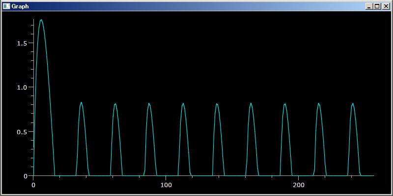
PythonSf ワンライナー


# 入力電流:Vi と出力電圧:Vx

sy(); f0=50Hz`; f=7V` absF(sin(2pi f0 `T)); C,Rs,Rl=1000uF`, 1Ω`,33Ω`;mt=kOde(λ t,Vx:[1,((f(t)-Vx)/Rs-Vx/Rl)/C if f(t)>=Vx else (-Vx/Rl)/C],[0,0],100ms`,256); plotGr([(f(t)-Vx)/Rs if f(t)>=Vx else 0 for t,Vx in mt]);plotGr(mt[:,1],color=red)
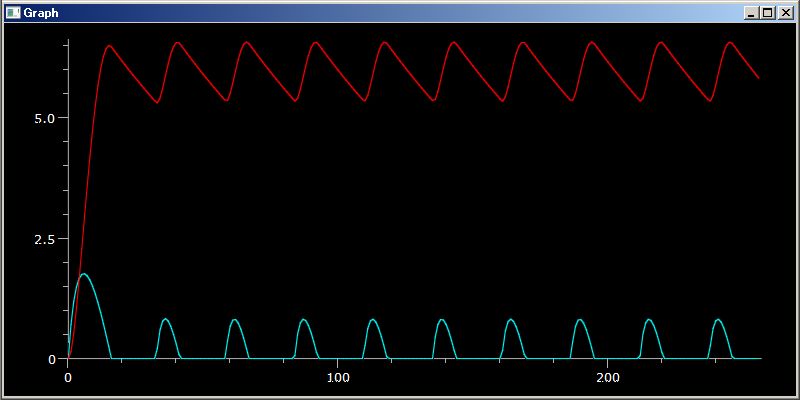
縦軸が電圧値と電流値の両方を兼ねています。単位が異なります。物理的には許されません。でも自分だけが見るグラフならば、意味が分っていますから許されるでしょう。
PythonSf ワンライナー


# 最大突入電流:Vi

sy(); f0=50Hz`; f=7V` absF(cos(2pi f0 `T)); C,Rs,Rl=1000uF`, 1Ω`,33Ω`;mt=kOde(λ t,Vx:[1,((f(t)-Vx)/Rs-Vx/Rl)/C if f(t)>=Vx else (-Vx/Rl)/C],[0,0],100ms`,256); plotGr([(f(t)-Vx)/Rs if f(t)>=Vx else 0 for t,Vx in mt])
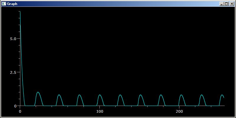
最大突入電流を計算するため、入力電圧関数を sin(.) ではなく cos(.) にしました。
シリコンの 0.6V 分も含めた計算も簡単です。λ式を二重に使い、キーワード引数を O'Caml などの let 文の代わりにしています。
PythonSf ワンライナー


sy(); f0=50Hz`; f=λ t:(λ v=7V` cos(2pi f0 t):v-0.6V` if v>0.6V` else 0)(); C,Rs,Rl=1000uF`, 1Ω`,33Ω`;mt=kOde(λ t,Vx:[1,((f(t)-Vx)/Rs-Vx/Rl)/C if f(t)>=Vx else (-Vx/Rl)/C],[0,0],100ms`,256); plotGr([(f(t)-Vx)/Rs if f(t)>=Vx else 0 for t,Vx in mt])
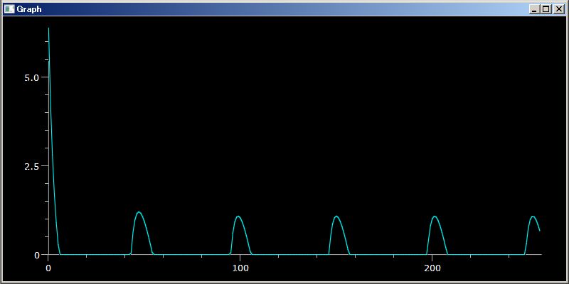
PythonSf には、ラプラス演算子 s に対応する有理関数クラスの単項式 `s が備わっています。`s は z 変換の単項式としても扱えます。。これを使えばアナログ・フィルタ、デジタル・フィルタの挙動が短い PythonSf ワン・ライナー式で簡単に計算できます。Matlab,Mathematica など他の数学ソフトでは、ここまで簡単には計算できないと思います。以下の one-liners を見てやってください。
標準配布の PythonSf に備わっている `s を使えば、回路の Laplace 演算子を使った式を扱えます。そのボード線図、インパルス応答、インディシャル応答が簡単に求められます。この `s を使って下の L C R を組み合わせた回路の動作を検討してみましょう。
L C R 回路
                      11mH       10Ω
            Vi ──∩∩∩∩ ─WMWM─┐ ──→ Vo
                                    │
                                  ─┴─
                                  ─┬─
                                    │1uF
                                    │
                                    Ξ
コイル L は微分要素であり、その Lapalace 演算子表現は L `s です。C は積分要素であり、その Laplace 演算子表現は 1/(C `s) です。ですから L C R 三つを直列につないだときの impedence の Laplace 演算子表現 (L `s + 1/(C `s) + R) となります。
ですから、上の回路の電圧伝達関数 Vo/Vi は下のように PythonSf 式で計算できます。この伝達関数を何回か再利用するため、ファイル変数 G としてカレント・ディレクトリに残すことも、下の PythonSf 式の G:= ... の式で行わせています。
PythonSf ワンライナー
L,C,R=1000uH`, 1uF`, 10Ω`; G:=1/(C `s)/(L `s + 1/(C `s) + R)
===============================

       1e+09
-------------------
 2
s + 1e+04 s + 1e+09
この伝達関数 G が どんなものか Python に備わっている自己ドキュメント機能を使って調べてみましょう。
PythonSf ワンライナーたち
# G は どんなクラス? ----- ClRtnl クラス
=:G; type(G)
===============================
<class 'pysf.rational.ClRtnl'>

# ClRtnl はどんなメソッドを備えている?
np.info(ClRtnl)
 ClRtnl(numerAg, denomAg=1, variable='s')

' Ratianal Function class
    The highest coefficient of demoninator is always 1
'


Methods:

  getAnRspns  --
  getDgRspns  --
  deriv  --  Return the derivative of this rational funciton.
  plotDgGnPh  --
  getAnImpls  --
  plotBode  --
  getRtnlOfRtnl  --
  getDgImpls  --
  plotAnRspns  --
===============================
None

# G が保持しているデータは? ---- 分母と分子の多項式
=:G; vars(G)
===============================
{'m_plNumer': poly1d([  1.00000000e+09]), 'm_plDenom': poly1d([  1.00000000e+00,   1.00000000e+04,   1.00000000e+09])}
G は plotBode(..) 関数を備えています。この関数で Bode 線図を描きます。名前から Bode 線図を描かせる関数だと分かります。どんな使い方をするのでしょうか調べましょう。
PythonSf ワンライナー
# ClRtnl:plotBode 関数の使い方を調べる
=:G; np.info(G.plotBode)
 plotBode(lowerFreq, higherFreq=None)

'  plot Bode diagram using matplotlib
    Default frequency width is 3 decades
'
===============================
None
Bode 線図を描かせるには周波数範囲を指定してやる必要があるようです。伝達関数 G は m_plDenon: poly1d 多項式のインスタンスを備えています。ならば、その根が判れば Bode 線図の周波数範囲も決まります。
PythonSf ワンライナー
=:G; G.m_plDenom.roots
===============================
[-5000.+31224.98999199j -5000.-31224.98999199j]
上の計算結果:分母多項式の根は 3kHz 周波数近辺に共振することを示しています。ならば その二桁下 10Hz から二桁上 100kHz の範囲の周波数でボード線図を描けば良さそうです。
PythonSf ワンライナー
=:G; G.plotBode(10Hz`, 100k` Hz`)
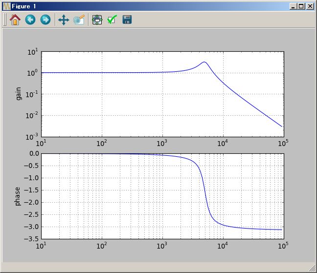
plotAnImpls(..) 関数を使って、上の回路のインパルス応答を見てみましょう。グラフの時間表示範囲は 3kHz より判断して、時間の範囲は 0 -- 2ms としましょう。
PythonSf ワンライナー
=:G; plotGr(G.getAnImpls( 2ms`))
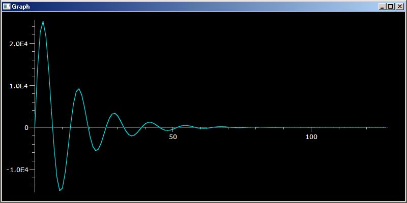
PythonSf ワンライナー
=:G; G.()
インパルス応答の次は plotAnRspns(..) メソッドを使ってステップ応答を見てみましょう。
PythonSf ワンライナー
=:G; G.plotAnRspns( 2ms`)
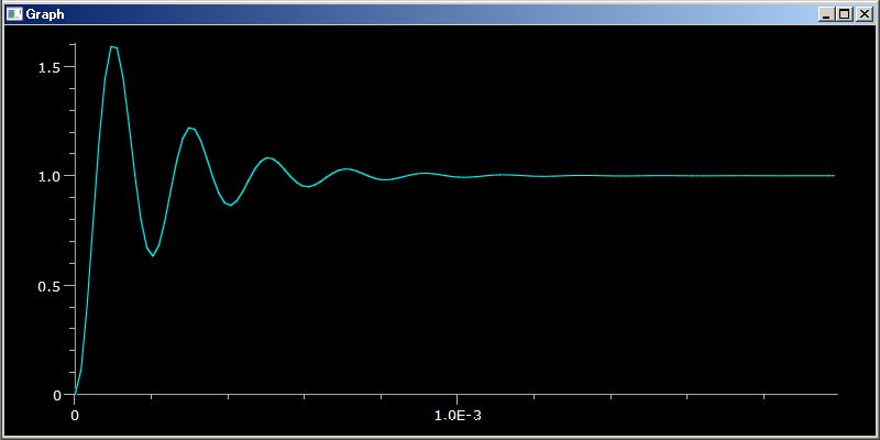
今度は上の回路に 1kHz 正弦波を入力したときの応答をみてみましょう。 1kHz 正弦波関数は sin(2pi 1k` Hz` `T) と記述できます。(0,2ms) の区間を 256 等分したベクトル・データは klsp(0,2ms`,256) で作れます。これを引数にして sin(2pi 1k` Hz` `T)(klsp(0,2ms`,256) を計算してやれば、ikHz 正弦波の 2ms までの 256 点のベクトル・データが得られます。このデータを上の .getAnRspns(..) の二番目の引数に与えれやれば、上の回路に正弦波入力を与えたときの応答が得られます。
PythonSf ワンライナー
=:G;G.plotAnRspns(2ms`,sin(2pi 1k` Hz` `T)(klsp(0,2ms`, 256)))
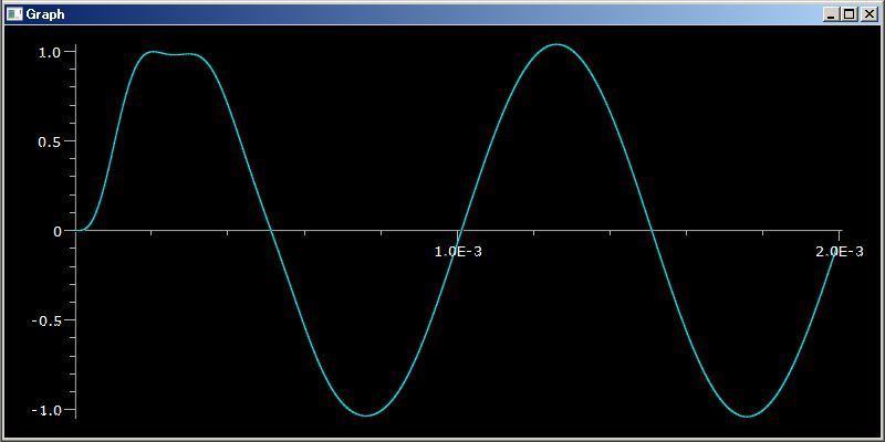
コンデンサ 1uF に充電が完了するまでの時間:初期の 0.5ms までは L C 共振成分が見られますが、それ以後は 1kHz の正弦波になっています。
ちなみに、矩形波入力を入れたときは次のような応答波形になります
PythonSf ワンライナー
=:G;G.plotAnRspns(2ms`,[(λ t:-1-2np.floor(2 (-0.5+ t 1k` Hz` -int(t 1k` Hz`)) ))(x) for x in klsp(0,2ms`, 256)])
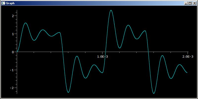
上の PythonSf 式で矩形波を作っている λ t:-1-2np.floor(2 (-0.5+ t 1k` Hz` -int(t 1k` Hz`)) ) が少しく技巧的です。こんなのは、すらすらとは出てこないでしょう。矩形波を表す関数を手続き的にプログラムするべきかもしれません。実際には下のような順序で導出しています。こっちは関数プログラミング的な導出方だと思います。こちらの方が数学的思考に集中できます。手続き的なプログラム作成に伴うデバッグが入らないからです。
PythonSf ワンライナーたち
plotGr(λ t: t-int(t 1k` Hz`), 0,10ms`)
plotGr(λ t: t 1k` Hz` -int(t 1k` Hz`), 0,10ms`)
plotGr(λ t: np.floor(2 (-0.5+ t 1k` Hz` -int(t 1k` Hz`)) ), 0,10ms`)
plotGr(λ t: np.floor(2 (-0.5+ t 1k` Hz` -int(t 1k` Hz`)) ), 0,2.5ms`)
plotGr([(λ t: np.floor(2 (-0.4+ t 1k` Hz` -int(t 1k` Hz`)) ))(x) for x in klsp(0,2ms`, 256)])
plotGr([(λ t: np.floor(2 (-0.5+ t 1k` Hz` -int(t 1k` Hz`)) ))(x) for x in klsp(0,2ms`, 256)])
plotGr([(λ t: 1+2np.floor(2 (-0.5+ t 1k` Hz` -int(t 1k` Hz`)) ))(x) for x in klsp(0,2ms`, 256)])
plotGr([(λ t:-1-2np.floor(2 (-0.5+ t 1k` Hz` -int(t 1k` Hz`)) ))(x) for x in klsp(0,2ms`, 256)])
RIAA 回路
         R1:82kΩ                R3:1kΩ
────WMWM───┬──────WMWM────┬────
                  │                        │
                  ≧                        │
                  ≦R2:12kΩ                │
                  │                        │
                ─┴─                    ─┴─
                ─┬─ C1:0.027uF         ─┬─ C2:8200pF
                  │                        │
─────────┴────────────┴────
ここでは二端子網回路の F 行列を使って、上の RIAA 回路の電圧伝達関数を計算します。
標準配布 PythonSf の sfCrrntIni.py には、直列接続または並列接続の二端子網回路の F 行列を返す Fs(.) と Fp(.) が実装されています。これを使えば、上の RIAA 回路の R1 直列抵抗や R1 + 1/(C1 `s) 並列要素の F 行列は下のように計算できます。
PythonSf ワンライナーたち
R1=82kΩ`;  Fs(R1)
===============================
[[ClRtnl([ 1.],[ 1.]), ClRtnl([ 0.],[1])],
       [ClRtnl([-82000.],[ 1.]), ClRtnl([ 1.],[ 1.])]]
---- ClFldTns:< class 'pysf.rational.ClRtnl'> ----

R2,C1=12kΩ`,0.027uF`; Fp(R2+1/(C1 `s))
===============================
[[ClRtnl([ 1.],[ 1.]),
        ClRtnl([ -8.33333333e-05,   0.00000000e+00],[  1.00000000e+00,   3.08641975e+03])],
       [ClRtnl([ 0.],[1]), ClRtnl([ 1.],[ 1.])]]
---- ClFldTns:< class 'pysf.rational.ClRtnl'> ----
RIAA 回路の要素ごとに F 行列が求められるのならば、それを掛け合わせてやれば RIAA 回路の F 行列が計算できます。下のような具合です。
PythonSf ワンライナー
R1,R2,R3,C1,C2=82kΩ`,12kΩ`,1kΩ`,0.027uF`,8200pF`;  Fp(1/(C2 `s)) Fs(R3) Fp(R2+1/(C1 `s)) Fs(R1)
===============================
[[ ClRtnl([  7.36633333e-04,   9.93395062e+00,   3.08641975e+03],[  1.00000000e+00,   3.08641975e+03]),
        ClRtnl([ -8.88333333e-09,  -1.08641975e-04,   0.00000000e+00],[  1.00000000e+00,   3.08641975e+03])],
       [ ClRtnl([ -8.98333333e+04,  -2.56172840e+08],[  1.00000000e+00,   3.08641975e+03]),
        ClRtnl([  1.08333333e+00,   3.08641975e+03],[  1.00000000e+00,   3.08641975e+03])]]
---- ClFldTns:< class 'pysf.rational.ClRtnl'> ----
F 行列が定まれば、その電圧伝達関数は -F[1,0] F[0,1]/F[0,0] + F[1,1] で計算できます。下のような具合です。
PythonSf ワンライナーたち
R1,R2,R3,C1,C2=82kΩ`,12kΩ`,1kΩ`,0.027uF`,8200pF`;F=Fp(1/(C2 `s)) Fs(R3) Fp(R2+1/(C1 `s)) Fs(R1);(-F[1,0] F[0,1]/F[0,0] + F[1,1])
===============================
           3             2
     1358 s + 1.257e+07 s + 3.88e+10 s + 3.991e+13
-------------------------------------------------------
 4             3             2
s + 1.966e+04 s + 9.696e+07 s + 1.543e+11 s + 3.991e+13


R1,R2,R3,C1,C2=82kΩ`,12kΩ`,1kΩ`,0.027uF`,8200pF`;F=Fp(1/(C2 `s)) Fs(R3) Fp(R2+1/(C1 `s)) Fs(R1);(-F[1,0] F[0,1]/F[0,0] + F[1,1]).plotBode(1Hz`,100k` Hz`)
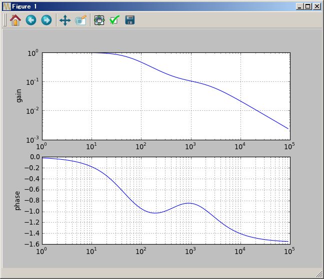
F 行列以外に Z 行列 Y 行列 などを返す関数を作ってやれば任意トポロジーの伝達関数を計算できるようになると思いますが、そこまでは実装していません。回路のプロのどなたか、この実装をしてみませんか。理屈さえわかっていれば、それらの実装は簡単です。Fs(.), Fp(.) 関数は下のような超が付くほどの簡単な実装で済んでいます。
PythonSf ワンライナー
np.source(Fs)
In file: sfCrrntIni.py

Fs = lambda Z:sf.krry__(*[[1.0,0.0],[-Z*1.0,1.0], sf.ClRtnl])

===============================
None

PythonSf ワンライナー
np.source(Fp)
In file: sfCrrntIni.py

Fp = lambda Z:sf.krry__(*[[1.0,-1.0/Z],[0.0,1.0], sf.ClRtnl])

===============================
None
`s を作っているクラス ClRtnl には、デジタル・フィルタ向けのインパルスも応答関数:getDgImpls(..)、ステップ応答・一般応答関数:getDgRspns(.;)、ゲイン・位相表示関数:plotDgGnPh(..) も備えています。ですから下のような z 変換を使った算計処理が可能です。
PythonSf ワンライナー
# FIR インパルス応答
z_=1/`s; (z_^1 + 2z_^2+ 3z_^3).getDgImpls()[:10]
===============================
[ 0.  1.  2.  3.  0.  0.  0.  0.  0.  0.]
---- ClTensor ----

PythonSf ワンライナー
# FIR ステップ応答
z_=1/`s; (z_^1 + 2z_^2+ 3z_^3).getDgRspns()[:10]
===============================
[ 0.  1.  3.  6.  6.  6.  6.  6.  6.  6.]

PythonSf ワンライナー
# IIR ステップ応答
z=`s; ((z +1)/(z^1 + 2z^2+ 3z^3)).getDgImpls()[:10]
===============================
[ 0.          0.          0.33333333  0.11111111 -0.18518519  0.08641975
  0.00411523 -0.03155007  0.01966164 -0.00259107]
---- ClTensor ----

PythonSf ワンライナー
# IIR ゲイン・位相図の描画
z=`s; (z^-1 + 2z^-2+ 3z^-3).plotDgGnPh()
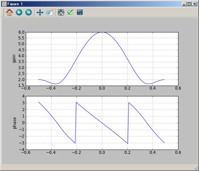
置換群 Sn(N) を実装しました。ただし群論に詳しくない素人の愚直な実装であり、計算時間を短くする対策が入っていません。N が 10 を超えた Sn(N) 置換群全体を iterate 処理させると計算に何時間もかかってしまいます。でも N が 8 ぐらいまでならば Sn(8) 全部を実用的に iterate することもできます。これぐらいまでの処理でも多くの有限群の性質を確認できます。これならば学部での群論の勉強には十分だと考えています。
標準配布の sfCrrntIni.py には置換群インスタンスのクラス:Sb、巡回置換インスタンスを返す関数 Cy、置換群インスタンスを要素とする frozenset クラス:kfs(..)、群生成関数:grp(..) をグローバル変数として定義し直してあるので、PythonSf 式で直接に使えます。 また標準配布のディレクトリには置換群の集合インスタンス SS2,SS3,SS4,SS5、交代群の集合インスタンス SA3,SA4 のファイル変数を置いてあります。 これぐらい用意されていれば初等的な群論の検討には不便ないでしょう。
数学ソフトに詳しい方は「GAP を使えよ」と仰ると思います。同意します。複雑な群論の処理、大規模な対象を扱うときは GAP を使うべきです。でも Sn(8) ぐらいまでの小規模な群までならば、vim などから PythonSf 式で扱える Sb, Cy, ksf, grp のほうが便利です。以下の PythonSf 式による群の扱いを見てください。
以下有限置換群 Sn(N) を扱う Sb,Cy,group,kfs といったクラスや関数の詳細を見ていきます。
Sb(...) は 0 から n までの整数を並べ替えたシーケンスを引数に与えることで置換インスタンスを作ります。この並べ替えたシーケンス引数は、多変数引数として与えます。またリストあるいはタプル引数でも与えられます。
PythonSf ワンライナーたち
# 多変数引数
Sb(1,3,2,0)
===============================
Sb(1,3,2,0)

# リスト引数
x=[1,3,2,0]; Sb(x)
===============================
Sb(1,3,2,0)

# タプル引数
x=(1,3,2,0); Sb(x)
===============================
Sb(1,3,2,0)
Sb インスタンスどうしの掛け算と Sb インスタンスへの整数べき乗算が可能です。長さの異なる Sb インスタンスの積も可能です。下のような PythonSf 式として置換インスタンスの計算を扱えます。
PythonSf ワンライナーたち
# Sb インスタンスどうしの積
a,b=Sb(1,3,2,0), Sb(3,0,2,1); a b
===============================
Sb(0,1,2,3)

# Sb インスタンスの 2 乗
Sb(1,3,2,0)^2
===============================
Sb(3,0,2,1)

# Sb インスタンスの -1 乗:逆元
Sb(1,3,2,0)^-1
===============================
Sb(3,0,2,1)

# Sb インスタンスの  2 乗
Sb(1,3,2,0)^-2
===============================
Sb(1,3,2,0)

# Sb インスタンスの  3 乗:単位元に戻る
Sb(1,3,2,0)^3
===============================
Sb(0,1,2,3)

# 異なる長さの Sb インスタンスの積
Sb(1,3,2,0) Sb(1,3,2,0,4)
===============================
Sb(3,0,2,1,4)

# 異なる長さの Sb インスタンスの積 2
Sb(1,3,2,0) Sb(1,4,2,0,3)
===============================
Sb(3,4,2,1,0)

# 巡回群リストの生成
a=Sb(1,3,2,0); [a^k for k in range(4)]
===============================
[Sb(0,1,2,3), Sb(1,3,2,0), Sb(3,0,2,1), Sb(0,1,2,3)]

# 長い Sb インスタンス
seed(0);Sb(shuffle(range(20)))
===============================
Sb(16,9,19,10,2,11,15,13,4,7,0,18,1,17,5,8,3,6,12,14)
Cy(..) 関数は巡回置換 Sb(..) インスタンスを返します。Sb(..) のときとは違って、必要な整数の組み合わせだけを引数に与えれば済むので、置換群の PythonSf 式の記述が簡単になることが多くあります。
PythonSf ワンライナーたち
Cy(1,2,3)
===============================
Sb(0,2,3,1)

Cy(1,3)
===============================
Sb(0,3,2,1)

Cy(1,3) Sb(range(10))
===============================
Sb(0,3,2,1,4,5,6,7,8,9)

# cyclic 属性
Sb(16,9,19,10,2,11,15,13,4,7,0,18,1,17,5,8,3,6,12,14).cyclic
===============================
Cy(0,16,3,10) Cy(1,9,7,13,17,6,15,8,4,2,19,14,5,11,18,12)

Cy(0,16,3,10) Cy(1,9,7,13,17,6,15,8,4,2,19,14,5,11,18,12)
===============================
Sb(16,9,19,10,2,11,15,13,4,7,0,18,1,17,5,8,3,6,12,14)

# 巡回群と互換の積
(Cy(0,2) Cy(2,4) Cy(4,1) Cy(1,8)).cyclic
===============================
Cy(0,2,4,1,8)

# 巡回群と Sn(N)
# Sn(4) == group([Cy(0,1),Cy(1,2),Cy(2,3)}
=:SS4; SS4 == group([Cy(0,1),Cy(1,2),Cy(2,3)])
===============================
True
Sb インスタンスを要素とする置換群の集合を扱うとき、その集合は frozenset の方が望ましいことが多くあります。関数で引き渡した先で変更されないことが保証されます。set のときのように copy/deep_copy に注意を払わなくて済むからです。そして置換要素の集合としての群は kfs:frozenset で扱うことに統一しておかないと、== 演算子での判断が面倒になってしまいます。
でも frozenset のスペルは PythonSf 式の one-liner 記述には長すぎます。そこで frozenset を継承した kfs クラスを設けました。ついでに kfs 集合の union(..) は + 演算子で可能にしました。kfs 集合の meet(..) は * 演算子で可能にしました。
ついでに frozenset を iterate するとき、その繰り返し順序が判らないと困ることが多いので sortedList:sl プロパティを設けて、sort 済みのリストを返すようにしました。これでデバッグが楽になります。ループ処理ごとに、どのインスタンスをを処理しているのかが判るからです。kfs(..) 集合をプリントするときも sorted 済みの結果で表示します。
PythonSf ワンライナーたち
# Sb インスタンスよりなる kfs 集合の生成
kfs([Sb(0,1), Sb(2,1,0)])
===============================
kfs([Sb(0,1), Sb(2,1,0)])

# 巡回群集合の生成
a=Sb(1,3,2,0); kfs( [a^k for k in range(4)] )
===============================
kfs([Sb(0,1,2,3), Sb(1,3,2,0), Sb(3,0,2,1)])

# 集合の和:union
a=Sb(1,3,2,0); b,c=kfs( [a^k for k in range(4)] ), kfs([Sb(0,1), Sb(2,1,0)]); b+c
===============================
kfs([Sb(0,1), Sb(2,1,0), Sb(0,1,2,3), Sb(1,3,2,0), Sb(3,0,2,1)])

# 集合の積:meet
a=Sb(1,3,2,0); b,c=kfs( [a^k for k in range(4)] ), kfs([Sb(0,1), Sb(3,0,2,1)]); b*c
===============================
kfs([Sb(3,0,2,1)])
ただし kfs クラスの要素にできるのは sort 可能なインスタンスに限られます。最後の結果をコンソールに質力するときに sort 作業がなされるからです。ですから整数・実数・複素要素値のベクトルや行列を要素とするkfs 集合は作れません。コンソールに出力するときの sorting でエラーになります。下のような具合です
PythonSf ワンライナー
kfs([~[1,2],~[3,4]])
===============================
The truth value of an array with more than one element is ambiguous. Use a.any() or a.all() at excecuting:kfs([krry__(*[1,2]),krry__(*[3,4])])

PythonSf ブロック実行
//@@
a=kfs([~[1,2],~[3,4]])
print a+5
//@@@
Traceback (most recent call last):
  File "__tempConverted.py", line 9, in
    print a+5
  File "D:\my\vc7\mtCm\pysf\ptGrp.py", line 432, in __str__
    return "kfs(" + str(self.sl) + ")"
  File "D:\my\vc7\mtCm\pysf\ptGrp.py", line 357, in __getattr__
    return sorted((self))
ValueError: The truth value of an array with more than one element is ambiguous. Use a.any() or a.all()
置換群の集合インスタンス SS2,SS3,SS4,SS5、交代群の集合インスタンス SA3,SA4 のファイル変数を、標準配布のカレント・ディレクトリに置いてあります。 これらは kfs クラスのインスタンスです。
PythonSf ワンライナーたち
=:SS3; SS3
===============================
kfs([Sb(0,1,2), Sb(0,2,1), Sb(1,0,2), Sb(1,2,0), Sb(2,0,1), Sb(2,1,0)])

=:SA3; SA3
===============================
kfs([Sb(0,1,2), Sb(1,2,0), Sb(2,0,1)])
群論の剰余類・共役類などを扱うのを容易にするため、kfs 集合インスタンスと 置換要素との積を可能にしています。同様な意味で kfs 集合インスタンスと要素との和も可能にしています。もちろん置換群の kfs 集合インスタンスと置換群要素の和演算は無意味でありエラーになります。でも整数集合などでは意味がある分野もあるでしょう。次のような PythonSf 式計算ができます。
PythonSf ワンライナーたち
# 置換集合と置換の積
a=Sb(1,3,2,0); SG=kfs( [a^k for k in range(4)] ); g=Sb(3,2,1,0); SG g
===============================
kfs([Sb(0,2,3,1), Sb(1,2,0,3), Sb(3,2,1,0)])

# 共役集合の計算 1
a=Sb(1,3,2,0); SG=kfs( [a^k for k in range(4)] ); g=Sb(3,2,1,0); g SG g^-1
===============================
kfs([Sb(0,1,2,3), Sb(2,1,3,0), Sb(3,1,0,2)])

# 共役集合の計算 2
a=Sb(1,3,2,0); SG=kfs( [a^k for k in range(4)] ); g=Sb(3,2,1,0); g^-1 SG g
===============================
kfs([Sb(0,1,2,3), Sb(2,1,3,0), Sb(3,1,0,2)])

# 整数集合と整数の積
kfs([1,2,3]) 4
===============================
kfs([4, 8, 12])

# 整数とタプルの集合と整数の積
kfs([1,  (2,3)]) 4
===============================
kfs([4, (2, 3, 2, 3, 2, 3, 2, 3)])

# 整数集合と整数の積
kfs([1,2,3]) + 4
===============================
kfs([5, 6, 7])
一つだけ kfs 要素が Sb インスタンスであることを前提としているのが / 演算子です。ksf 集合を、その部分集合で割ることで左剰余類群の集合を返します。この機能は kfs 要素が Sb 以外であると旨く働きません。
PythonSf ワンライナー
=:SS3,SA3; SS3/SA3
===============================
kfs([Sb(0,1,2), Sb(0,2,1)])
group(..) 関数の引数に Sb インスタンスのリスト or タプル or セットを与えると、その Sb インスタンスたちによって生成される群の kfs 集合を返します。下のような PythonSf 式が使えます。
PythonSf ワンライナーたち
# group({ Sb(1,0), Cy(range(N)}) による Sn(N) 置換群全体集合の生成
N=3; group({Sb(1,0),Cy(range(N))})
===============================
kfs([Sb(0,1,2), Sb(0,2,1), Sb(1,0,2), Sb(1,2,0), Sb(2,0,1), Sb(2,1,0)])

# group({ Sb(1,0), Cy(range(4)}) による置換群全体集合が Sn(4) であることの確認
=:SS4; N=4; group({Sb(1,0),Cy(range(N))}) == SS4
===============================
True
group(..) 関数は、全ての積の組み合わせで作られる集合を作ります。それにより集合の新たな要素が追加されなくなるまでリカーシブに新たに集合を作り直します。ですから Sn(N):N が 10 以上の長い Sb インスタンスを group(..) に渡してやると、それ返す集合要素数は n! となるかも知れません。そうなると一時間でも計算が終わらなくなるでしょう。ご注意ください。
PythonSf 有限群論の最後に交換子群を実際に計算してみます。
PythonSf ワンライナーたち
# SN(3) の交換子積の集合
SS=:SS3; {x y x^-1 y^-1 for x,y in mitr(SS,SS)}
===============================
set([Sb(0,1,2), Sb(1,2,0), Sb(2,0,1)])

# SN(3) の交換子群:交換子積の集合と同じ
SS=:SS3; group([x y x^-1 y^-1 for x,y in mitr(SS,SS)])
===============================
kfs([Sb(0,1,2), Sb(1,2,0), Sb(2,0,1)])

# SN(4) の交換子積の集合
SS=:SS4;   kfs([x y x^-1 y^-1 for x,y in mitr(SS,SS)])
===============================
kfs([Sb(0,1,2,3), Sb(0,2,3,1), Sb(0,3,1,2), Sb(1,0,3,2), Sb(1,2,0,3), Sb(1,3,2,0), Sb(2,0,1,3), Sb(2,1,3,0), Sb(2,3,0,1), Sb(3,0,2,1), Sb(3,1,0,2), Sb(3,2,1,0)])

# SN(4) の交換子群:交換子積の集合と同じ
SS=:SS4; group([x y x^-1 y^-1 for x,y in mitr(SS,SS)])
===============================
kfs([Sb(0,1,2,3), Sb(0,2,3,1), Sb(0,3,1,2), Sb(1,0,3,2), Sb(1,2,0,3), Sb(1,3,2,0), Sb(2,0,1,3), Sb(2,1,3,0), Sb(2,3,0,1), Sb(3,0,2,1), Sb(3,1,0,2), Sb(3,2,1,0)])

# SN(4) の交換子群は交代群:An(4) になる
SS=:SS4; =:SA4; group([x y x^-1 y^-1 for x,y in mitr(SS,SS)]) == SA4
===============================
True

# An(4) の交換子群
SS       =:SA4; group([x y x^-1 y^-1 for x,y in mitr(SS,SS)])
===============================
kfs([Sb(0,1,2,3), Sb(1,0,3,2), Sb(2,3,0,1), Sb(3,2,1,0)])
PythonSf を使うということは、Ramanujan 級の計算能力を得られたということです。この能力を使えば様々の分野で数学を使った遊びが可能になります。以下、その遊びの幾つかを見ていきましょう。
元の Maxima の式


plot3d((1/8)*(6*exp(-(((2/3)*abs(x) - 1)^2 + ((2/3)*y)^2) - (1/3)*((2/3)*y + (1/2))^3) + (2/3)*exp(-%e^11*( (abs((2/3)*x) - 1)^2 + ((2/3)*y)^2)^2) + (2/3)*y - ((2/3)*x)^4),


http://www.rainbowseeker.jp/xoops/modules/newbb/viewtopic.php?topic_id=369&forum=10&noreadjump=1


PythonSf ワンライナー


x,y,e=`X,`Y,exp(1); plot3dGr((1/8)*(6*exp(-(((2/3)*absF(x) - 1)^2 + ((2/3)*y)^2) - (1/3)*((2/3)*y + (1/2))^3) + (2/3)*exp(-e^11*( (absF((2/3)*x) - 1)^2 + ((2/3)*y)^2)^2) + (2/3)*y - ((2/3)*x)^4),klsp(-3,3,100))
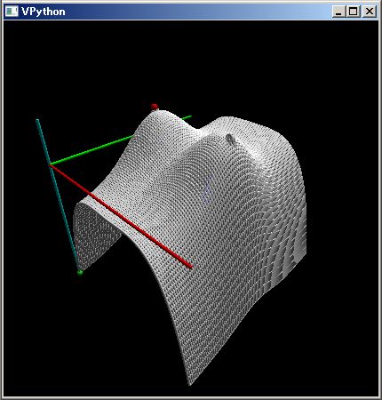
絶対値関数は Python に備わっている abs(..) 関数ではなく、PythonSf が用意している加減乗除べき乗算と関数合成が可能な absF(..) 関数を使います。 abs(..) 関数は python 文法に組み込まれており、これを呼び出すと引数オブジェクトの __abs__(self) method が呼び出されるからです。
なお左乳首が赤いのは意識してプログラムしたわけではありません。plot3dGr(..) は最初に出てくる最大値の位置に赤い丸を、最小値の位置に緑の丸を追加するため、左乳首の位置に赤い丸が置かれてしまいました。
フェルマーの最終定理:「n>=3 のとき x^n+y^n=z^n を満たす 0 でない自然数の組み合わせは存在しない」という定理は有名です。近年この問題は肯定的に証明されたようですが、素人に解る証明ではないでしょう。
単純な別証明なんて作れませんが、x^n + y^n よりは小さいが できるだけ近い z^n は存在するはずです。その z^n と x^n+y^n の差分がどんな分布をしているのか見てみましょう。n=3 のとき その分布は下の PythonSf ワン・ライナー式で計算できます。
PythonSf ワンライナー
N,n=16 ,3; ls=range(N); krry([ [(x^n+y^n)-((x^n+y^n+10^-9)^(1/n)//1)^n for x in ls] for y in ls], int)
===============================
[[  0   0   0   0   0   0   0   0   0   0   0   0   0   0   0   0]
 [  0   1   1   1   1   1   1   1   1   1   1   1   1   1   1   1]
 [  0   1   8   8   8   8   8   8   8   8   8   8   8   8   8   8]
 [  0   1   8  27  27  27  27  27  27  27  27  27  27  27  27  27]
 [  0   1   8  27   3  64  64  64  64  64  64  64  64  64  64  64]
 [  0   1   8  27  64  34 125 125 125 125 125 125 125 125 125 125]
 [  0   1   8  27  64 125  89  47 216 216 216 216 216 216 216 216]
 [  0   1   8  27  64 125  47 174 126  72  12 343 343 343 343 343]
 [  0   1   8  27  64 125 216 126  24 241 181 115  43 512 512 512]
 [  0   1   8  27  64 125 216  72 241 127   1 332 260 182  98   8]
 [  0   1   8  27  64 125 216  12 181   1 272 134 531 453 369 279]
 [  0   1   8  27  64 125 216 343 115 332 134 465 315 153 700 610]
 [  0   1   8  27  64 125 216 343  43 260 531 315  81 550 376 190]
 [  0   1   8  27  64 125 216 343 512 182 453 153 550 298  28 659]
 [  0   1   8  27  64 125 216 343 512  98 369 700 376  28 575 287]
 [  0   1   8  27  64 125 216 343 512   8 279 610 190 659 287 918]]
---- ClTensor ----
上の値分布は規則性を感じます。でも その規則を明晰には述べられません。N を 50 にまで広げて、その分布を三次元グラフとして表示してみましょう。
上の行列数値で感じたものに近い規則性があると思います。皆様は如何でしょうか。
PythonSf ワンライナー
N,n=50,3; ls=range(N); renderMtrx(krry([ [(x^n+y^n)-((x^n+y^n+10^-9)^(1/n)//1)^n for x in ls] for y in ls], int))
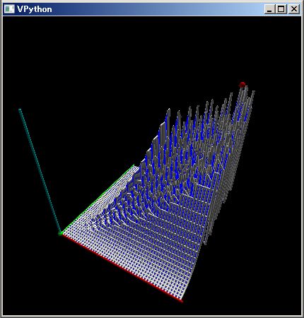
[0,1] 区間上のランダム値を返す rand(..) 関数, 平均値 0 分散 1 の正規分布ランダム値を返す randn(..) 関数、指定された範囲の整数値を返す randint(..) は、行列データも返せるので、手軽に様々な数値実験が可能です。その幾つかを示してみます。直感とは異なることも幾つかあるでしょう。ぜひとも、御自分の手で、様々の別パラメータ値で再実験をしてみてください。
1000 点の正規分布ノイズによる一次元の酔歩:Random Walk を下のように可視化できます。
PythonSf ワンライナー
#一次元の酔歩
N=1000; seed(0); lst=[0]; for v in randn(N):lst.append(lst[-1]+v); plotGr(lst)
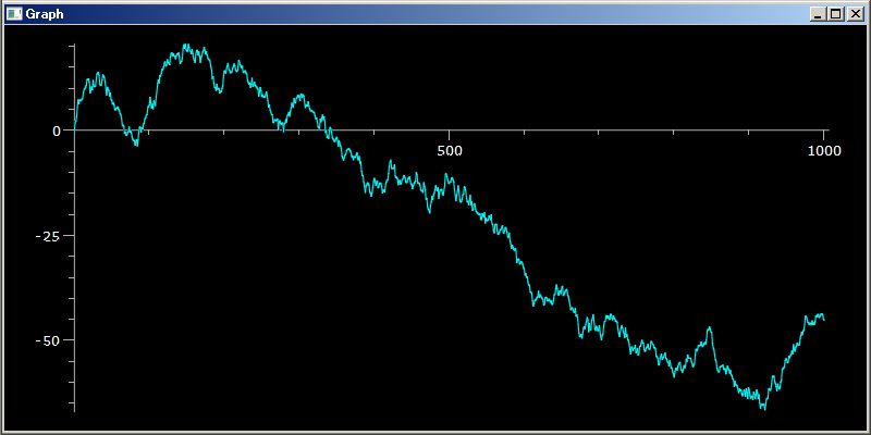
上の図は株価変動に似ています。でもランダムなノイズによる Random Walk なのに変化に傾向性があるのが気になります。上の図を株価のグラフとして見せられたら、値下がりのトレンドにあると見なしてしまいます。
Numpy の random 関数に誤りがありトレンドが出やすくなっているのでしょうか。それとも本当にランダムであっても上のグラフ程度のトレンドは簡単に現れるものなのでしょうか。
分からんときに何かを変えてやると別の視点から見れることが多くあります。1000 点の一様ノイズによる一次元の酔歩:Random Walk を見てみましょう
PythonSf ワンライナー
N=1000; seed(0); lst=[0]; for v in rand(N)-0.5:lst.append(lst[-1]+v); plotGr(lst)
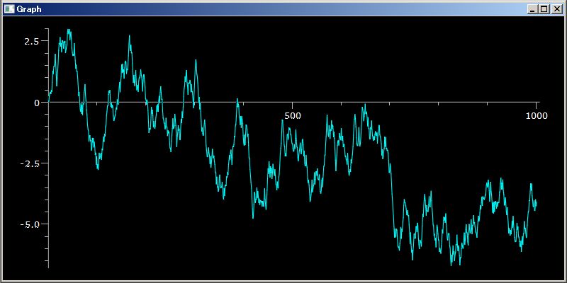
より変動が激しくなりました。これでもトレンドが伺えます。
もっと自然なランダム・データを使って、トレンドが出てくるかみれば、上のトレンドのようなものがランダムなデータにも出てくるか見えてくるはずです。円周率 1000 桁をランダムなデータとして Random Walk を描かせて見ましょう。
PythonSf ブロック
//@@
strData=(
"31415926535897932384626433832795028841971693993751058209749445923078164062862089986280348253421170679"
+"8214808651328230664709384460955058223172535940812848111745028410270193852110555964462294895493038196"
+"4428810975665933446128475648233786783165271201909145648566923460348610454326648213393607260249141273"
+"7245870066063155881748815209209628292540917153643678925903600113305305488204665213841469519415116094"
+"3305727036575959195309218611738193261179310511854807446237996274956735188575272489122793818301194912"
+"9833673362440656643086021394946395224737190702179860943702770539217176293176752384674818467669405132"
+"0005681271452635608277857713427577896091736371787214684409012249534301465495853710507922796892589235"
+"4201995611212902196086403441815981362977477130996051870721134999999837297804995105973173281609631859"
+"5024459455346908302642522308253344685035261931188171010003137838752886587533208381420617177669147303"
+"5982534904287554687311595628638823537875937519577818577805321712268066130019278766111959092164201989"
)

lst=[0]
#;; 4.5 == sum(range(10))/10
for ch in strData:lst.append(lst[-1]+int(ch)-4.5); plotGr(lst)
//@@@
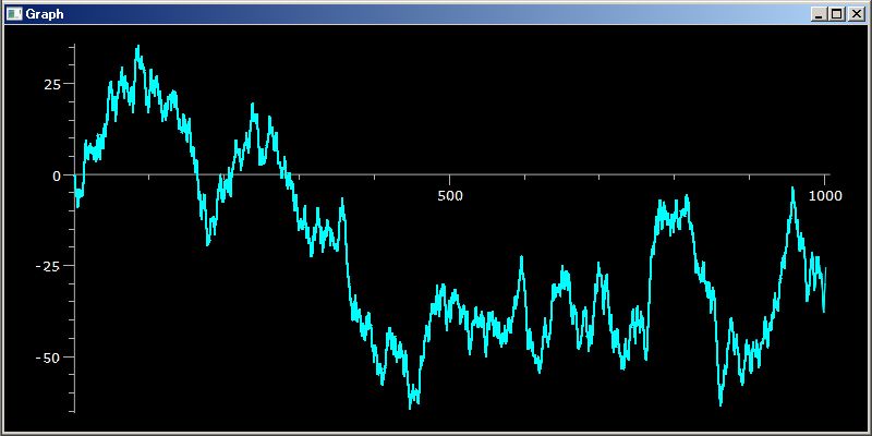
円周率にランダムではないなんらかの傾向性があれば誰かが発表しているはずですが、そんな話は見られません。上の 1000 点の円周率のデータは、自然なランダム・データだと思ってよいでしょう。
この円周率データによる一次元の酔歩:Random Walk でもトレンドのようなものが見られます。どうも株価でトレンドといっているものにはランダムであることに起因する偶然なものも多くありそうです。
皆様も seed(.) の引数値を変えるなどしてランダム・データによるトレンドの具合の変化を、自分で体験してみてください。
二次元、三次元の酔歩も容易に描けます。下のような具合です。
PythonSf ワンライナー
# 二次元の酔歩
N=1000; seed(0); lst=[~[0,0]]; for vc in randn(N,2):lst.append(lst[-1]+vc); plotTrajectory(lst)
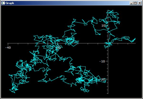
PythonSf ワンライナー
# 三次元の酔歩
N=1000; seed(0); lst=[~[0,0,0]]; for vc in randn(N,3):lst.append(lst[-1]+vc); plotTrajectory(lst)
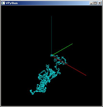
こんな図を見ていると、昔顕微鏡下の花粉の動きを生物としての動きと誤解したのも納得できます。
民生用の電子機器で使っている抵抗の大多数が、 3σ で 5% の精度のものです。1kΩ の抵抗を 10 個持ってきたら、その抵抗値のばらつきは正規分布に従うはずであり、以下のような具合になるはずです。
PythonSf ワンライナー
N=10; r,R=0.05, 1kΩ`; seed(0); R (1+ r/3 randn(N))
===============================
[ 1029.40087243  1006.66928681  1016.31229974  1037.34821999  1031.1259665
   983.71203534  1015.83480696   997.47737986   998.2796858   1006.84330837]
---- ClTensor ----
ちなみに 5% 以上の誤差になるものは、1000 個の抵抗のうちで 2 個ぐらいです。
PythonSf ワンライナー
N=1000; r,R=0.05, 1kΩ`; vc=R (1+ r/3 randn(N)); len([ x for x in vc if x<0.95R or 1.05R<x])
===============================
2
10% 以上の誤差になるものは1000000 個の抵抗持ってきても 0 個です。
PythonSf ワンライナー
N=1000000; r,R=0.05, 1kΩ`; vc=R (1+ r/3 randn(N)); len([ x for x in vc if x<0.9 R or 1.1 R<x])
===============================
0
以上の計算より、5% 3σ 精度の抵抗値は、500 個に一個程度 5% を超えるものがある。でも 100 万個の抵抗をもってきても 10% を超える誤差のものは出てこないといえます。
ちなみに、5% 抵抗を合成してやると、抵抗の誤差同士が打ち消しあって より少ない抵抗値のばらつきになります。
下の回路の合成抵抗値は並列接続で半分になり直接接続で倍になるので、全体としては 1kΩ に戻ります。
           1kΩ               1kΩ
       ┌─WMWM─┐      ┌─WMWM─┐
   ──┤        ├───┤        ├─
       │  1kΩ  │      │  1kΩ  │
       └─MWMW─┘      └─MWMW─┘
この回路の抵抗値 1kΩ のばらつき具合:標準偏差は下のようにシミュレーション計算できます。
PythonSf ワンライナー


N=1000; r,R=0.05, 1kΩ`; seed(0); vc=[ (vc1~+vc2)+(vc3~+vc4) for vc1,vc2,vc3,vc4 in R (1+ r/3 randn(N,4))]; sqrt( sum([ (x-sum(vc)/N)^2 for x in vc ])/(N-1) )

===============================

8.31846294487
元の標準偏差 1kΩ, 5%, 3σ から定まる抵抗値のばらつきぐあい 50/3 の半分程度のばらつきぐあいになりました。
「四次元立方体を三次元に射影する」ことを PythonSf で行います。でも最初からでは難しいので「三次元立方体を二次元に射影する」ことを行ってから、それを四次元に拡張する手順を踏みます。
PythonSf での one-liners を使って思考の螺旋階段を上っていく様子がよく分かる例だと思います。
三次元立方体の頂点は下の PythonSf 式で表現できます。
PythonSf ワンライナー

# 三次元立方体の頂点

ls=[-1,1]; [ ~[x,y,z] for x,y,z in mitr(ls,ls,ls)]

===============================

[ClTensor([-1., -1., -1.]), ClTensor([-1., -1.,  1.]), ClTensor([-1.,  1., -1.]), ClTensor([-1.,  1.,  1.]), ClTensor([ 1., -1., -1.]), ClTensor([ 1., -1.,  1.]), ClTensor([ 1.,  1., -1.]), ClTensor([ 1.,  1.,  1.])]
下の one-liner の方が、八個の頂点が分かりやすいですね。
PythonSf ワンライナー
# 2^3:八個の頂点
ls=[-1,1]; ~[ [x,y,z] for x,y,z in mitr(ls,ls,ls)]
===============================
[[-1. -1. -1.]
 [-1. -1.  1.]
 [-1.  1. -1.]
 [-1.  1.  1.]
 [ 1. -1. -1.]
 [ 1. -1.  1.]
 [ 1.  1. -1.]
 [ 1.  1.  1.]]
---- ClTensor ----
座標軸の原点一箇所から放出される光線が立方体の各頂点を通って平面と交わる点を求めることで、立方体を平面に射影できます。そのため Z 軸に垂直な射影される平面を想定します。その Z 軸との交点は 12 の位置にあるものとしましょう。
原点一箇所から放出される光線が、上で作った立方体の八個の頂点を通って平面に射影されるよう、 その立方体をZ 軸方向に 6 だけ平行移動させます。下の PythonSf 式を使って、カレント・ディレクトリの mt.pvl ファイルに、その頂点の座標値を残します。 。
PythonSf ワンライナー
ls=[-1,1]; mt:= ~[ ~[x,y,z] for x,y,z in mitr(ls,ls,ls)]+ ~[0,0,6]
===============================
[[-1. -1.  5.]
 [-1. -1.  7.]
 [-1.  1.  5.]
 [-1.  1.  7.]
 [ 1. -1.  5.]
 [ 1. -1.  7.]
 [ 1.  1.  5.]
 [ 1.  1.  7.]]
---- ClTensor ----
[0,0,0] 原点から放射された光線が、上で求めた八つの頂点を通って、上で想定した Z 軸に垂直な平面で交わったと想定し、その平面と直線の交点座標を求めましょう。
「Z 軸に直行し [0,0,12] で交わる平面」と「原点と ~[x,y,z] 点を通った直線」が交わる点の座標を求めます。
(t ~[x,y,z])[2] == 12 for ∃t
t z == 12
∴
t = 12/z for z ∈ {5,7}
ゆえに平面との交点の座標は下の PythonSf 式で計算できる
12/z ~[x,y,z]
具体例で再度考えましょう。「Z 軸に直行し [0,0,12] で交わる平面」と「原点と ~[-1,-1,7] 点を通った直線」が交わる点の座標は次の PythonSf 式で求められます。
PythonSf ワンライナー
12/7 ~[-1,-1,17]
===============================
[ -1.71428571 -1.71428571 29.14285714]
---- ClTensor ----
ですから、上で作った立方体の八つの頂点を通る、座標軸の原点から射出されて光線は下の八つの点で平面と交わります。この点は mt2dCube の名前のファイル変数で保存します。
PythonSf ワンライナー
=:mt; mt2dCube:=~[ v 12/v[2] for v in mt]
===============================
[[ -2.4 -2.4 12. ]
[ -1.71428571 -1.71428571 12. ]
[ -2.4 2.4 12. ]
[ -1.71428571 1.71428571 12. ]
[ 2.4 -2.4 12. ]
[ 1.71428571 -1.71428571 12. ]
[ 2.4 2.4 12. ]
[ 1.71428571 1.71428571 12. ]]
---- ClTensor ----
ファイル変数 mt, mt2dCube それぞれ八つの座標位置を人間に分かりやすいように、下の PytthonSf 式を使って図示します。
PythonSf ワンライナー
mt,mt2=:mt,mt2dCube; for v0,v1 in combinate(mt,2):plotTrajectory([v0,v1]); for v0,v1 in combinate(mt2,2):plotTrajectory([v0,v1],color=red);
上の図で赤い部分が立方体の射影図です。
三次元の立方体を平面に射影することと殆ど同様に、四次元立方体を四次元の超平面:三次元空間に射影できます。
四次元立方体の 2^4:16 個の頂点を、第4の 軸方向に 6 だけ平行移動させたときの頂点の座標をファイル変数 mt に残します。
PythonSf ワンライナー
ls=[-1,1]; mt:= ~[ ~[x,y,z,t] for x,y,z,t in mitr(ls,ls,ls,ls)]+ ~[0,0,0,6]
===============================
[[-1. -1. -1. 5.]
[-1. -1. -1. 7.]
[-1. -1. 1. 5.]
[-1. -1. 1. 7.]
[-1. 1. -1. 5.]
[-1. 1. -1. 7.]
[-1. 1. 1. 5.]
[-1. 1. 1. 7.]
[ 1. -1. -1. 5.]
[ 1. -1. -1. 7.]
[ 1. -1. 1. 5.]
[ 1. -1. 1. 7.]
[ 1. 1. -1. 5.]
[ 1. 1. -1. 7.]
[ 1. 1. 1. 5.]
[ 1. 1. 1. 7.]]
---- ClTensor ----
第四の軸に直行し [0,0,0,12] で交わる超平面に、原点と立方体の頂点を通る直線が交わる座標を求め、ファイル変数 mt3dCube に残します。
PythonSf ワンライナー
=:mt; mt3dCube:=~[ v 12/v[3] for v in mt]
===============================
[[ -2.4 -2.4 -2.4 12. ]
[ -1.71428571 -1.71428571 -1.71428571 12. ]
[ -2.4 -2.4 2.4 12. ]
[ -1.71428571 -1.71428571 1.71428571 12. ]
[ -2.4 2.4 -2.4 12. ]
[ -1.71428571 1.71428571 -1.71428571 12. ]
[ -2.4 2.4 2.4 12. ]
[ -1.71428571 1.71428571 1.71428571 12. ]
[ 2.4 -2.4 -2.4 12. ]
[ 1.71428571 -1.71428571 -1.71428571 12. ]
[ 2.4 -2.4 2.4 12. ]
[ 1.71428571 -1.71428571 1.71428571 12. ]
[ 2.4 2.4 -2.4 12. ]
[ 1.71428571 1.71428571 -1.71428571 12. ]
[ 2.4 2.4 2.4 12. ]
[ 1.71428571 1.71428571 1.71428571 12. ]]
---- ClTensor ----
四次元での超平面:すなわち三次元空間に射影された四次元立方体の三次元図を下の PythonSf 式で描きます。
PythonSf ワンライナー
mt=:mt3dCube; [plotTrajectory([v0[:3],v1[:3]])for v0,v1 in combinate(mt,2) if norm(v0-v1)~==4.8 or norm(v0-v1)~==(2*1.71428571)]
五次元立方体を四次元超平面に射影し、その四次元立体をさらに三次元空間に射影したときの頂点の位置も次の PythonSf 式で描けます。
PythonSf ワンライナー
ls=[-1,1]; mt= ~[ v for v in mitr(*[ls]*5)]+ ~[0,0,0,0,6];mt=~[ v 12/v[4] for v in mt][:,:-1]+[0,0,0,6]; mt=~[ v 12/v[3] for v in mt][:,:-1];plotPt(mt); drawAxis()
こんな図形は自分の手で回転させ様々の方向から見てみないと分かりにくいと思います。ぜひ上の one-liner で御自分のコンピュータで動かしマウスで動かしてみてください。
ここで行った立方体を平面に、四次元立方体を三次元に射影する PythonSf 式たちは、プログラム・コードを書いているのではなく、数式を書き連ねていると言ったほうが近いと思います。プログラム・コード記述の苦しさが殆どありません。面倒なプログラム・デバッグもありません。数学思考に集中できます。途中までの計算結果を見ながら PythonSf 式を書き連らねているだけです。
Python の正規表現は使いにくすぎます。Perl でのような正規表現を使いまくるコードを書く気にはなれません。正規表現をコンパイルしてから チェックする文字列に match(...) させ group(..) で取り出すなんて面倒なことをしてられません。そこで kre.py 正規表現改良モジュールを作りました。正規表現にマッチング・インスタンスを「対象文字列 / 正規表現」と割り算演算子で返すようにしました。部分文字列を「%(序数)」mod 演算子で返すようにしました。「対象文字列 / 正規表現%0」で正規表現にマッチした文字列を返すようにしました。
PythonSf では krgl('正規表現文字列') でコンパイル済みの正規表現インスタンスを作ります。これで対象文字列を割ってやれば、正規表現処理されたマッチング・インスタンスができます。これを %0 でわれば、マッチする文字列が帰ります。次のような具合です。
PythonSf ワンライナーたち
'abcdefg'/krgl('[c-e]*')%0
===============================
cde
'abcdefghijkl'/krgl('([c-e]*).*([g-i]+)')%0
===============================
abcdefghi
'abcdefghijkl'/krgl('([c-e]+).*([g-i]+)')%1
===============================
cde
'abcdefghijkl'/krgl('([c-e]*).*([g-i]+)')%2
===============================
i
PythonSf 正規表現クラス krgl を使えばワンライナーで実用的なことが様々にできます。次のような具合です。
PythonSf ワンライナーたち
# pysf ディレクリとにあるファイルのうち k で始まるファイル名のものを列挙します
rg,wlk=krgl('^k'),os.walk('./pysf'); `print( [(path,[f for f in files if f/rg%0]) for path,dir,files in wlk] )
[('./pysf',
['kcommon.py',
'kcommon.pyc',
'kmayavi.py',
'kmayavi.pyc',
'kmayaviPy.bak',
'kNumeric.bak',
'kNumeric.py',
'kNumeric.pyc',
'kNumericPy.bak',
'kre.py',
'kre.pyc'])]
===============================
None
# PythonSf の実行時に定まっているグローバル変数の中から plot で始まるものを列挙する
# PythonSf のグローバル変数で不正確に記憶している名称を探すのに便利です
rg=krgl('^plot'); [ s for s in globals().keys() if s/rg%0]
===============================
['plot3dGr', 'plotTmCh', 'plot3d', 'plotPt', 'plotBode', 'plotTrajectory', 'plot2d', 'plot3dRowCol', 'plotGr', 'plotDgGnPh']
# SymPy モジュールのグローバル変数全体から fact を含むものを列挙する
# kre.se.I 引数を追加することで大文字/小文字を区別させない
import sympy as md; rg=krgl('fact',kre.se.I); [ s for s in vars(md).keys() if s/rg%0]
===============================
['factorint', 'factorial2', 'cofactors', 'factorial', 'factor_', 'factor', 'factortools', 'FallingFactorial', 'primefactors', 'factor_list', 'RisingFactorial', 'facts']
このように kre.py の正規表現クラス krgl 使えば、 Perl でのような正規表現の活用の仕方が可能になります。 `
PythonSf では Oc(...) を使うことで、四元数、八元数を扱えます。Cayley/Dicson 構成法:八元数操作を Zp(N) 有元体に適用してやることで、非可換または結合率の成り立たない有限代数系が使えるようになります。
PythonSf には八元数:Octornion:oc.Oc を備えており、非可換な代数での挙動、結合率さえ成り立たない代数での挙動を簡単にコンピュータ上で実行させ試してみることができりす。八元数 oc.Oc だといっても、上側の数値が 0 のときは、それを表示しないので、引数を四つ以下に限定にしてやれば quaternion としての動作になります。引数を二つ以下に限定してやれば複素数の動作になります。
Oc(1,2,3,4,5) Oc(5,0,7)
===============================
Oc(-16, -18, 22, 34, 25, 0, -35, 0)
Oc(1,2,3,4) Oc(5,6,7,8)
===============================
Oc(-60, 12, 30, 24)
Oc(1,2 ) Oc(5,6 )
===============================
Oc(-7, 16)
この oc.Oc の八元数演算の実装は、愚直に積と和の組み合わせ演算だけでなされています。ですから oc.Oc に 実数以外の体インスタンスを渡してやれば、その一般体の上で、八元数の加減乗除算が実行されてしまいます。すなわち一般体複素数、一般体四元数、一般体八元数の演算が行われるように代数系を拡張できてしまいます。
体の八元数化による体代数系の拡張はCayley_Dickson_construction ,「ケーリー=ディクソンの構成法」として知られています。
ケーリー=ディクソンの構成法の良いところは拡張された代数系の挙動の予測が付けやすいことです。足し算については、元の体代数系のベクトル足し算になります。積演算については、四元数にしてやることで非可換な代数系が得られます。八元数にしてやることで結合律さえ成り立たない代数系が得られます。
このケーリー=ディクソンの構成法を Zp(N) に適用してやれば、簡単に非可換であったり結合律が成り立たない有限な代数系を作れます。そして有限:小規模な代数系ならばコンピュータで虱潰しに調べ上げられるので便利です。といっても、実際にそのようなプログラムを 0 から作り上げるのは普通の人間では月単位の仕事になってしまうでしょう。でも PythonSf ならば八元数の要素を Zp(N) 要素にしてやるだけで、それを実装できしまいます。
ClOctonion による「ケーリー=ディクソンの構成法」の適用は、まだ実験的な実装段階です。Compatibility のない仕様変更が将来なされる可能性があります。
PythonSf ワンライナー
# 非可換な例
O3(1,2,3,0) O3(2,1,0,1)
===============================
Oc(0, 2, 1, 1)
O3(2,1,0,1) O3(1,2,3,0)
===============================
Oc(0, 2, 2, 1)
# 非可換な例を虱潰しに挙げる
lst=[0,1,2]; mi=list( mitr(*([lst]*4)) ); [(tpL,tpR) for tpL,tpR in mitr(mi,mi) if O3(tpL) O3(tpR) != O3(tpR) O3(tpL)]
たくさん
# 可換な例を虱潰しに挙げる
lst=[0,1,2]; mi=list( mitr(*([lst]*4)) ); [(tpL,tpR) for tpL,tpR in mitr(mi,mi) if O3(tpL) O3(tpR) == O3(tpR) O3(tpL)]
たくさん
# 積演算の逆元
1/O3(1,0,2,3)
===============================
(2, 0, 2, 0)
# 逆元が存在しない例
1/O3(1,1,2,3)
snipped
ZeroDivisionError: Square value is 0 at ClOctonion:inv().
# ゼロ因子の例
O3(0,1,1,1) O3(2,0,1,2)
===============================
0
# ゼロ因子を虱潰しに挙げる
# λ x: O3(0,1,1,1) x の Kernel
# 積の単位元は含まれていない
ls=range(3); [ tpl for tpl in mitr(*[ls]*4) if O3(0,1,1,1) O3(tpl) == 0]
===============================
[(0, 0, 0, 0), (0, 1, 1, 1), (0, 2, 2, 2), (1, 0, 2, 1), (1, 1, 0, 2), (1, 2, 1, 0), (2, 0, 1, 2), (2, 1, 2, 0), (2, 2, 0, 1)]
# λ x: O3(0,1,1,1) x の Kernel は積演算について閉じている
ls=range(3); lst=[ tpl for tpl in mitr(*[ls]*4) if O3(0,1,1,1) O3(tpl) == 0]; [ O3(x) O3(y) in lst for x,y in mitr(lst,lst)]
===============================
[True, True, True, True, True, True, True, True, True, True, True, True, True, True, True, True, True, True, True, True, True, True, True, True, True, True, True, True, True, True, True, True, True, True, True, True, True, True, True, True, True, True, True, True, True, True, True, True, True, True, True, True, True, True, True, True, True, True, True, True, True, True, True, True, True, True, True, True, True, True, True, True, True, True, True, True, True, True, True, True, True]
# λ x: O3(0,1,1,1) x の Kernel は和演算について閉じている
ls=range(3); lst=[ tpl for tpl in mitr(*[ls]*4) if O3(0,1,1,1) O3(tpl) == 0]; [ O3(x)+O3(y) in lst for x,y in mitr(lst,lst)]
===============================
[True, True, True, True, True, True, True, True, True, True, True, True, True, True, True, True, True, True, True, True, True, True, True, True, True, True, True, True, True, True, True, True, True, True, True, True, True, True, True, True, True, True, True, True, True, True, True, True, True, True, True, True, True, True, True, True, True, True, True, True, True, True, True, True, True, True, True, True, True, True, True, True, True, True, True, True, True, True, True, True, True]
# この小さい環の世界でも非可換性は残っている
ls=range(3); lst=[ tpl for tpl in mitr(*[ls]*4) if O3(0,1,1,1) O3(tpl) == 0]; [ O3(x) O3(y) == O3(y) O3(x)in lst for x,y in mitr(lst,lst)]
===============================
[True, True, True, True, True, True, True, True, True, True, True, True, False, False, False, False, False, False, True, True, True, False, False, False, False, False, False, True, False, False, True, False, False, True, False, False, True, False, False, False, True, False, False, False, True, True, False, False, False, False, True, False, True, False, True, False, False, True, False, False, True, False, False, True, False, False, False, False, True, False, True, False, True, False, False, False, True, False, False, False, True]
下の fO5toO3 は O5 から O3 への自然変換とみなせる
PythonSf ワンライナー
fO5toO3 = fCT(λ x:O3(x.m_tpl), O5, O3); fO5toO3(O5(1,2,3,4))
===============================
(1, 2, 0, 1)
fO5toO3 = fCT(λ x:O3(x.m_tpl), O5, O3); fO5toO3.dom, fO5toO3.cod
===============================
((,), (,))
fO5toO3 = fCT(λ x:O3(x.m_tpl), O5, O3); fO5toO3(O3(1,2,6,4))
Traceback (most recent call last):
File "C:\Python27\lib\runpy.py", line 162, in _run_module_as_main
"__main__", fname, loader, pkg_name)
File "C:\Python27\lib\runpy.py", line 72, in _run_code
exec code in run_globals
File "D:\my\vc7\mtCm\sfPP.py", line 2, in
pysf.sfPPrcssr.start()
File "pysf\sfPPrcssr.py", line 2739, in start
__execLine( (" ".join(sys.argv[1:])).strip() )
File "pysf\sfPPrcssr.py", line 2355, in __execLine
valStt = eval(ustConvertedAt, globals(), locals() )
File "", line 1, in
File "sfCrrntIni.py", line 155, in _
+ str(sqAg[k])
File "sfCrrntIni.py", line 37, in Assert
raise sf.ClAppError(strAg)
pysf.sfFnctns.ClAppError: Error at CT:__call__(..) input type check:(1, 2, 0, 1)
product, sum も非自明な自然変換に使える
PythonSf ワンライナー
sum(O3(1,2,3,4))
===============================
1
product(O3(1,2,3,4))
===============================
0
product(O3(1,2,1,4))
===============================
0
<== 八元数での product になっている。下のようにせねばならない。
product(O3(1,2,1,4)[:4])
===============================
2
PythonSf ワンライナー
# 結合律が成り立たない整数八元数の例
O=oc.Oc; a,b,c=O(1,2,3,4,5),O(2,1,4,5,6),O(3,4,1,6,7); str((a b) c), str(a (b c))
===============================
('(-426, -279, 12, -323, -366, -4, 52, 12)', '(-426, -279, 12, -323, -366, -12, 44, -28)')
# 結合律が成り立たない Zp(3) 八元数の例
O=oc.Oc; a,b,c=O(~[1,2,3,4,5,Z3]),O(~[2,1,4,5,6,Z3]),O(~[3,4,1,6,7,Z3]); str((a b) c), str(a (b c))
===============================
('(0, 0, 0, 1, 0, 2, 1, 0)', '(0, 0, 0, 1, 0, 0, 2, 2)')
標準配布のカレント・ディレクトリの sfCrrntIni.py ファイルには圏論を扱うための dom, cod を扱えるようにする CT クラス、関数 fCT(..) が実装されています。圏論で頻出する monoid 構造を扱うため:即ち二項関数を扱うための関数 f2CT(..) も設けてあります。また~% user 演算子を関数合成操作に割り当ててあります。さらに Z2,Z3,Z4,Z5,Z5 有限体クラス、 O2,O3,O4,O5,O7 有限八元数クラスを設けてあり、圏論における様々の実例を実際に計算できる PythonSf one-liner 式で表現できます。
クラス CT は関数の入出力パラメータのタイプを指定するクラスです。Python でも、C や Java 言語での float function(int) のような、関数の型指定を可能にします。CT(int,float) で int 引数の float 出力の関数型指定を行うクラスのインスタンスを作ります。
PythonSf ワンライナー
CT(int, float)
===============================
このインスタンスに対し関数を渡してやると、int 引数を与えて、float 結果を返すことを確認する作業が追加された関数を返します。int を与えて float が返る動作をしているときは、下のように普通の動作をします。
PythonSf ワンライナー
ct=CT(int, float); f=ct(λ x:x+1.5); f(3)
===============================
4.5
でも、入力パラメータまたは出力結果の型が指定と異なるとき、次のように例外が発生します。
PythonSf ワンライナー
ct=CT(int, float); f=ct(λ x:x+1.5); f(3.1)
Traceback (most recent call last):
File "C:\Python27\lib\runpy.py", line 162, in _run_module_as_main
"__main__", fname, loader, pkg_name)
File "C:\Python27\lib\runpy.py", line 72, in _run_code
exec code in run_globals
File "D:\my\vc7\mtCm\sfPP.py", line 2, in
pysf.sfPPrcssr.start()
File "pysf\sfPPrcssr.py", line 2741, in start
__execLine( (" ".join(sys.argv[1:])).strip() )
File "pysf\sfPPrcssr.py", line 2357, in __execLine
valStt = eval(ustConvertedAt, globals(), locals() )
File "", line 1, in
File "sfCrrntIni.py", line 230, in _
+ str(sqAg[k])
File "sfCrrntIni.py", line 85, in Assert
raise sf.ClAppError(strAg)
pysf.sfFnctns.ClAppError: Error at CT:__call__(..) input type check:3.1
入力引数や戻り値の型は、リストで型を指定することで複数の引数値に対応させます。また型指定には集合や True/False 値を返す関数を使うことも可能です。下のような具合です
PythonSf ワンライナー
ct=CT([int, float,{7,8,9},λ x:isinstance(x,complex)], complex); f=ct(λ x,y,z,t:x+y+z+6+1.5j); f(3,4.1, 7, 2j)
===============================
(20.1+1.5j)
ct=CT([int, float,{7,8,9},λ x:isinstance(x,complex)], complex); f=ct(λ x,y,z,t:x+y+z+6+1.5j); f(3,4.1, 5, 2j)
Traceback (most recent call last):
File "C:\Python27\lib\runpy.py", line 162, in _run_module_as_main
"__main__", fname, loader, pkg_name)
File "C:\Python27\lib\runpy.py", line 72, in _run_code
exec code in run_globals
File "D:\my\vc7\mtCm\sfPP.py", line 2, in
pysf.sfPPrcssr.start()
File "pysf\sfPPrcssr.py", line 2741, in start
__execLine( (" ".join(sys.argv[1:])).strip() )
File "pysf\sfPPrcssr.py", line 2357, in __execLine
valStt = eval(ustConvertedAt, globals(), locals() )
File "", line 1, in
File "sfCrrntIni.py", line 230, in _
+ str(sqAg[k])
File "sfCrrntIni.py", line 85, in Assert
raise sf.ClAppError(strAg)
pysf.sfFnctns.ClAppError: Error at CT:__call__(..) input type check:5
、その constructor で
上の CT クラスによる型指定機能は、圏論の dom/cod を明示するのに役立ちます。でもワン・ライナーで使うには CT クラスのインスタンスを毎度作らねばならず面倒です。なので下のような fCT(...) 関数を設けてあります。
PythonSf ワンライナー
np.source(fCT)
In file: sfCrrntIni.py
def fCT(f, inputTypeOrSqTypeAg=None, outTypeAg=None):
ctAt = CT(inputTypeOrSqTypeAg, outTypeAg)
return ctAt(f)
===============================
None
下のように使います。ちなみに type がデフォルトの None で指定されているときは、型チェックを行わないことを意味します。
PythonSf ワンライナーたち
f=fCT(λ x:x+1, Z3); f(Z3(2))
===============================
Z3(0)
f=fCT(λ x:x+1.5, int); f(0)
===============================
1.5
圏論で頻出する monoid のために二項関数の型指定を行う f2CT(..) も sfCrrntIn.py に実装しています。
PythonSf ワンライナー
np.source(f2CT)
In file: sfCrrntIni.py
def f2CT(f, ty=None, tyOut=None):
# comment
if ty==None and tyOut==None:
return fCT(f,[None,None],tyOut)
elif ty!=None and tyOut==None:
return fCT(f, [ty,ty], ty)
else:
# ty!=None and tyOut!=None:
return fCT(f, [ty,ty], tyOut)
===============================
None
下のように使います。ちなみに f2CT(..) のときは、戻り値の型をデフォルト None のままにしておくことは、戻り値の型が入力値の型と同じであることを意味しています。
PythonSf ワンライナーたち
f=f2CT(λ x,y:x+y, Z3); f(Z3(1), Z3(2))
===============================
Z3(0)
f=f2CT(λ x,y:x+y, Z3); f.dom, f.cod
===============================
((, ), (,))
f=f2CT(λ x,y:x+y+0.5, int, float); f(1, 2)
===============================
3.5
f=f2CT(λ x,y:x+y, int, float); f(1, 2)
Traceback (most recent call last):
File "C:\Python27\lib\runpy.py", line 162, in _run_module_as_main
"__main__", fname, loader, pkg_name)
File "C:\Python27\lib\runpy.py", line 72, in _run_code
exec code in run_globals
File "D:\my\vc7\mtCm\sfPP.py", line 2, in
pysf.sfPPrcssr.start()
File "pysf\sfPPrcssr.py", line 2741, in start
__execLine( (" ".join(sys.argv[1:])).strip() )
File "pysf\sfPPrcssr.py", line 2357, in __execLine
valStt = eval(ustConvertedAt, globals(), locals() )
File "", line 1, in
File "sfCrrntIni.py", line 256, in _
+ str(valAt)
File "sfCrrntIni.py", line 85, in Assert
raise sf.ClAppError(strAg)
pysf.sfFnctns.ClAppError: Error at CT:__call__(..) output type check:3
CT クラスを使って関数の入出力型を指定できることは、圏論の dom/cod を明示する意味で便利です。でも C/C++/Java でのように、プログラム全体に渡る整合性の確認を行わせる型指定の便利さまでは享受できません。Python では全ての関数で型指定・チェックが行われるわけではないからです。CT に過度に期待すべきではありません。また圏論での PythonSf 式による検討で、型チェックを行わずに済ますことも多くあります。
圏論の議論では Curry 化関数になっている CT クラスの fst,lst メンバーのほうが、型指定よりも便利に使えるかもしれません。fst は最初の引数の、lst は最後の引数の Curry 化関数です。次のように使います。
PythonSf ワンライナーたち
f=f2CT(λ x,y:x+2y, Z3); [f.fst(Z3(1))(Z3(x)) for x in range(5)]
===============================
[1, 0, 2, 1, 0]
f=f2CT(λ x,y:x+2y, Z3); [f.lst(Z3(1))(Z3(x)) for x in range(5)]
===============================
[2, 0, 1, 2, 0]
圏論で頻出する関数合成のために sfCrrntIni.py で、ユーザー演算子:~% に関数合成の機能をアサインしてあります。下のコードで実装されています。
# ~%: user 演算子に関数合成
k__tilda__UsOp_mul____ = lambda x,y:Oc(sf.krry((Oc(x) * Oc(y)).m_tpl, Z5)) # ~*
abstract nonsence と揶揄されることもある圏論なんかを、何が嬉しくてやるのかと言えば、集合論が弱すぎるからです。集合論では対象の構造を論じるのに {式(x) for x in ... } しかありません。あとは自然言語で記述していくことになります。
圏論は集合に結合律を満たす arrow 構造を追加します。これにより対象の構造を視覚化できます。数学の世界では広く出てくる結合律による縛りが、豊富なグラフ構造をもたらします。
その具体例として McLane の教科書の最初に書いてある直積集合の圏論的な扱いについてみてみましょう。ここの 4 ページで読めます。
集合論の範囲で {1,2} と {5,6,7} の直積集合は {(x,y) such that x∈{1,2},y∈{5,6,7} } とでも書くでしょう。PythonSf ならば次のように書けます。
PythonSf ワンライナー
# 集合 X,Y の直積集合 XxY を PythonSf 式で作る
X,Y={1,2},{5,6,7}; XxY={(x,y) for x,y in mitr(X,Y)}; XxY
===============================
set([(2, 7), (2, 6), (1, 5), (1, 6), (1, 7), (2, 5)])
# XxY を kfs frozenset にしてみる
X,Y={1,2},{5,6,7}; XxY=kfs([(x,y) for x,y in mitr(X,Y)]); XxY
===============================
kfs([(1, 5), (1, 6), (1, 7), (2, 5), (2, 6), (2, 7)])
(kfs:frozenset を使うと、その集合の中身が sorting されているので便利です。一方で {... ..} の集合記述も数学での表記に近く、記述も簡素です。以下では両方の集合記述が混在されて使われます。)
集合論での直積集合は要素ペアが示されるだけです。その働きは自然言語で不明瞭に説明されるだけです。集合論は数学的対象を記述する道具として弱すぎます。下のような、直積集合:XxYから X への自明な写像は明白だからと説明もされないことのほうが多いでしょう。
PythonSf ワンライナー
X,Y={1,2},{5,6,7}; XxY=kfs([(x,y) for x,y in mitr(X,Y)]); fXxY_X=fCT(λ tpl:tpl[0], XxY, X); fXxY_X((1,5))
===============================
1
圏論では集合 X と Y の直積集合 XxY は下のグラフで視覚化される、arrow p,q を伴った構造だと定義されます。
圏論での直積集合 XxY
{1,2} p q {5,6,7}
X ←─ XxY ──→ Y
↑ ↑ ↑
│ │∃!h │
│ │ │
└───W ────┘
f g
すなわち「(集合:XxY, arrow:p, arrow:q) が集合 X,Y の直積集合である」とは「任意の集合 W と f:W→X, g:W→Y 関数が与えられたとき、h:W→XxY がユニークに存在し f == h〇p, g== h〇q とできる」ことであるとされます。
こんな抽象的な言葉だけでは普通の人間では正しく理解できません。PythonSf を使って具体例を作ってみましょう。X,Y={1,2},{5,6,7} 二つの直積集合 XxY を dom とし、X,Y を cod とする p,q arrow 関数を下のように与えることで、圏論的な直積集合の定義の具体例を作れます。
PythonSf ワンライナー
X,Y={1,2},{5,6,7}; XxY=kfs([(x,y) for x,y in mitr(X,Y)]);p,q=fCT(λ x_y:x_y[0],XxY,X), fCT(λ x_y:x_y[1],XxY,Y)
===============================
(, )
上の XxY,p,q に対し、下のように W={0,1} 集合と arrow f,g を下のように与えてみます。
PythonSf ワンライナー
X,Y={1,2},{5,6,7}; XxY=kfs([(x,y) for x,y in mitr(X,Y)]);p,q=fCT(λ x_y:x_y[0],XxY,X), fCT(λ x_y:x_y[1],XxY,Y); W={10,11}; f,g=fCT(λ x:1,W,X), fCT(λ x:5+x%2,W,Y)
===============================
(<function _ at 0x02C6F430>, <function _ at 0x02C6F3B0>)
X,Y={1,2},{5,6,7}; XxY=kfs([(x,y) for x,y in mitr(X,Y)]);p,q=fCT(λ x_y:x_y[0],XxY,X), fCT(λ x_y:x_y[1],XxY,Y); W={10,11}; f,g=fCT(λ x:1,W,X), fCT(λ x:5+x%2,W,Y); [f(x) for x in W]
===============================
[1, 1]
X,Y={1,2},{5,6,7}; XxY=kfs([(x,y) for x,y in mitr(X,Y)]);p,q=fCT(λ x_y:x_y[0],XxY,X), fCT(λ x_y:x_y[1],XxY,Y); W={10,11}; f,g=fCT(λ x:1,W,X), fCT(λ x:5+x%2,W,Y); [g(x) for x in W]
===============================
[5, 6]
この適当に与えられた W,f,g に対し次のような ∃!h:W→XxY を作れます。
PythonSf ワンライナー
X,Y={1,2},{5,6,7}; XxY=kfs([(x,y) for x,y in mitr(X,Y)]);p,q=fCT(λ x_y:x_y[0],XxY,X), fCT(λ x_y:x_y[1],XxY,Y); W={10,11}; f,g=fCT(λ x:1,W,X), fCT(λ x:5+x%2,W,Y); dh={10:(1,5),11:(1,6)}; h=fCT(λ x:dh[x],W,XxY); [h(x) for x in W]
===============================
[(1, 5), (1, 6)]
このように与えられた h に対し先の直積集合のグラフが成り立つこと:arrow が commute することを次のように確認できます
PythonSf ワンライナーたち
# f と p〇h が commute する
X,Y={1,2},{5,6,7}; XxY=kfs([(x,y) for x,y in mitr(X,Y)]);p,q=fCT(λ x_y:x_y[0],XxY,X), fCT(λ x_y:x_y[1],XxY,Y); W={10,11}; f,g=fCT(λ x:1,W,X), fCT(λ x:5+x%2,W,Y); dh={10:(1,5),11:(1,6)}; h=fCT(λ x:dh[x],W,XxY); [f(x) == (p~%h)(x) for x in W]
===============================
[True, True]
# g と q〇h が commute する
X,Y={1,2},{5,6,7}; XxY=kfs([(x,y) for x,y in mitr(X,Y)]);p,q=fCT(λ x_y:x_y[0],XxY,X), fCT(λ x_y:x_y[1],XxY,Y); W={10,11}; f,g=fCT(λ x:1,W,X), fCT(λ x:5+x%2,W,Y); dh={10:(1,5),11:(1,6)}; h=fCT(λ x:dh[x],W,XxY); [g(x) == (q~%h)(x) for x in W]
===============================
[True, True]
この h 関数:arrow が与えられた W,f,g に対してユニークに定まることは虱潰しによる確認で証明できます。でも煩雑になりすぎるので省略します。自明に近いとも思います。
圏論の直積集合の定義ならば、集合 WW:{0,1,2,3,4,5} も X,Y の直積集合にできます。次のような pp,qq を考えて見ましょう。
# 圏論での直積集合
{0,1,2,3,4,5,6}
{1,2} pp qq {5,6,7}
X ←─ WW ──→ Y
↑ ↑ ↑
│ │∃!h │
│ │ │
└───W ────┘
f g
PythonSf ワンライナー
# pp:WW→X
X,Y={1,2},{5,6,7}; WW=kfs(range(6));pp,qq=fCT(λ x_y:1 if x_y<3 else 2,WW,X), fCT(λ x_y:5+x_y%3,WW,Y); W={10,11}; [pp(x) for x in WW]
===============================
[1, 1, 1, 2, 2, 2]
# qq:WW→Y
X,Y={1,2},{5,6,7}; WW=kfs(range(6));pp,qq=fCT(λ x_y:1 if x_y<3 else 2,WW,X), fCT(λ x_y:5+x_y%3,WW,Y); W={10,11}; [qq(x) for x in WW]
===============================
[5, 6, 7, 5, 6, 7]
上のような X,Y,WW,pp,qq に対し、先ほどの f,g に対応する ∃!h を次のように定義しましょう
PythonSf ワンライナー
X,Y={1,2},{5,6,7}; WW=kfs(range(6));pp,qq=fCT(λ x_y:1 if x_y<3 else 2,WW,X), fCT(λ x_y:5+x_y%3,WW,Y); W={10,11}; f,g=fCT(λ x:1,W,X), fCT(λ x:5+x%2,W,Y); dh={10:0,11:1}; h=fCT(λ x:dh[x],W,WW); [h(x) for x in W]
===============================
[0, 1]
上の ∃!h と {0,1,2,3,4,5} に対し、下のように直積構造が成立することを確認できます。
PythonSf ワンライナー
# f と pp〇h が commute する
X,Y={1,2},{5,6,7}; WW=kfs(range(6));pp,qq=fCT(λ x_y:1 if x_y<3 else 2,WW,X), fCT(λ x_y:5+x_y%3,WW,Y); W={10,11}; f,g=fCT(λ x:1,W,X), fCT(λ x:5+x%2,W,Y); dh={10:0,11:1}; h=fCT(λ x:dh[x],W,WW); [f(x)==(pp~%h)(x) for x in W]
===============================
[True, True]
# g と qq〇h が commute する
X,Y={1,2},{5,6,7}; WW=kfs(range(6));pp,qq=fCT(λ x_y:1 if x_y<3 else 2,WW,X), fCT(λ x_y:5+x_y%3,WW,Y); W={10,11}; f,g=fCT(λ x:1,W,X), fCT(λ x:5+x%2,W,Y); dh={10:0,11:1}; h=fCT(λ x:dh[x],W,WW); [g(x)==(qq~%h)(x) for x in W]
===============================
[True, True]
圏論の直積集合の定義を導入することで {0,1,2,3,4,5} のような直積集合とは思えない集合も {1,2} と {5,6,7} の直積集合とみなせるようになりました。これにより直積集合に関する多くの性質が {0,1,2,3,4,5} 集合についても成り立ちます。このことは {0,1,2,3,4,5} 集合に直積集合の構造を導入したとも言えます。圏論の威力を示す例だとも思います。皆様はどのように思われるでしょうか。
A──→ A + B ←─→B
│ l[f,g] │
│ V │
└──→ B ←──┘
to be discussed
圏論を使うことで、複数の分野に散在していた抽象概念を、さらなる高みから統一して把握しなおすことが可能になります。これは研究者などの「新たな概念を生み出す」者たちに強力なツールをもたらします。抽象的に頭の中だけでボンヤリと考えていたことがらにグラフを使って可視化された具体的な全体構造を見通せるようになります。
圏論は大学の研究者に限らす「新たな概念を生み出す」者たち全てが利用できる強力ツールです。例えば PythonSf の基本関数たち(sin, cos や `X 恒等関数など)は「リカーシブに加減乗除算と整数べき乗算が可能」です。この「リカーシブに加減乗除と整数べき乗算が可能」な構造は monad とみなせます。「リカーシブに加減乗除算と整数べき乗算が可能」にしているのは ClAF クラスの実装です。この実装仕様を定めるのに monad 構造を意識しているか否かは全体を見通すと力に決定的な違いをもたらします。
圏論なんて abstract nonsence だと思われている方もいると思います。でも「新たな概念を生み出す者」であることを望むならば、学んでおくべき新しい道具です。それを学ぶ手間隙以上の強力な道具を手に入れられます。
下の回路の伝達関数を考えます。
┌──┐
┌─┤ Zf ├─┐
│ └──┘ │
┌─┐→│Vm │
Vi ─┤Zi├─┴─◆- │
└─┘Ii │G >──┴─── Vo
┌─◇+
│
│
≡
下の関係式がなりたちます。
Vo = -G Vm ----------- (1)
Vi-Vm = Zi Ii --------- (2)
Vm - Vo = Zf Ii ------- (3)
Vo/Vi の伝達関数が欲しいので、下の PythonSf 式で symbolic な代数解を計算させます。
PythonSf ワンライナー
ts(); Vi,Vo,Vm, Ii, Zi,Zf, G = ts.symbols('Vi,Vo,Vm, Ii, Zi,Zf, G'); ts.solve([ts.Eq(Vo+G Vm), ts.Eq(Vi-Vm-Zi Ii), ts.Eq(Vm-Vo-Zf Ii)], [Vo,Vm,Ii])
===============================
{Vo: G*Vi*Zf/(-G*Zi - Zf - Zi), Ii: Vi*(G + 1)/(G*Zi + Zf + Zi), Vm: Vi*Zf/(G*Zi + Zf + Zi)}
上の代数解より、Vo と Vi には下の関係式が成り立つことが解ります。
Vo==-G Vi Zf/(G Zi + Zf + Zi)
==- Vi Zf/( Zi + (Zf + Zi)/G ) --------- (4)
∴
Vo/Vi == -Zf/(Zi + (Zf + Zi)/G ) ----------- (5)
G が無限大のとき
Vo/Vi == -Zf/Zi ----------------------------- (6)
さて代表的なオペアンプ uA741 の DC ゲインは 25000 倍であり、その GBW は 1MHz です。そのファイル変数 uA741.pvl を下のように作っておきましょう。後で上の G に代入する形で使います。
PythonSf ワンライナー
f=1 M` Hz`; uA741:=2pi f/(`s + 2pi f/25000)
===============================
6.283e+06
---------
s + 251.3
PythonSf ワンライナー
G=:uA741; G.plotBode(0.1Hz`, 10M` Hz`)
下のような回路の特性を検討してみましょう
C1:0.001uF
┌──┤├──┐
│ R2:10kΩ │
├──MWMW──┤
Ii R1:1kΩ C1:0.1uF│ │
───MWMW──┤├──┴─◆- │
Vi Vm │ G>──┴───
┌─◇+ uA741
│
│
≡
理想オペアンプのとき、(6) 式より、上の回路の周波数特性は次のようになります。(下の式で ~+ 演算子は並列接続での足し算を計算させています)
PythonSf ワンライナー
R1,R2,C1,C2=1kΩ`,10kΩ`,0.1uF`,0.001uF`; Zi,Zf = R1+1/(C1 `s), R2~+(1/(C2 `s)); (-Zf/Zi ).plotBode(10 Hz`, 10 M` Hz`)
uA741 オペアンプのとき、(5)式より上の回路の周波数特性は次のようになります。ゲイン特性が 1MHz 近辺で異なります。位相特性は、100kHz ぐらいから違ってきています。
PythonSf ワンライナー
G=:uA741; R1,R2,C1,C2=1kΩ`,10kΩ`,0.1uF`,0.001uF`; Zi,Zf = R1+1/(C1 `s), R2~+(1/(C2 `s)); ( -Zf/(Zi + (Zf + Zi)/G ) ).plotBode(10 Hz`, 10 M` Hz`)
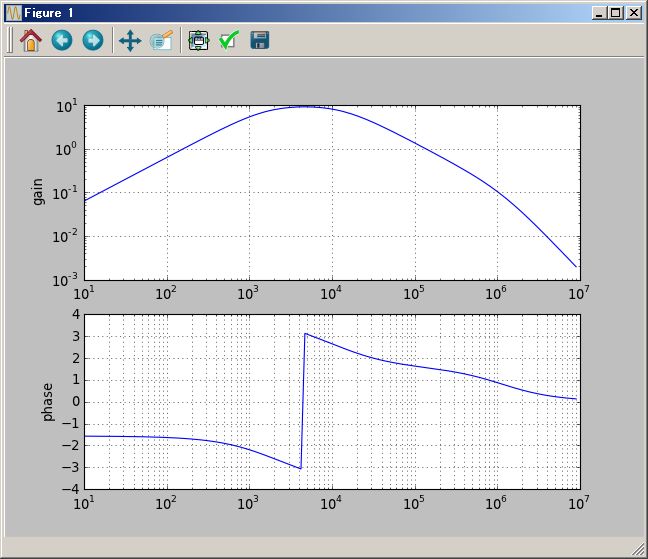
理想オペアンプと uA741 でのステップ応答の違いを見てみましょう
PythonSf ワンライナー
G=:uA741; R1,R2,C1,C2=1kΩ`,10kΩ`,0.1uF`,0.001uF`; Zi,Zf = R1+1/(C1 `s), R2~+(1/(C2 `s)); ( -Zf/Zi ).plotAnRspns(0.3ms`); ( -Zf/(Zi + (Zf + Zi)/G ) ).plotAnRspns(0.3ms`, color=red)
赤い線のほうが uA741 側です。当然ながら uA741 のステップ応答のほうが少し鈍ります。でも多くの場合で許されそうな範囲です。
厳密には uA741 の slew rate は 0.5V/us 程度ですから、そっちの方の影響の方が少しだけ強そうです。もし slew rate まで含めてシミュレートしようとすると、PythonSf ではなく Spice を持ち出してくるべきでしょう。PythonSf でも kOde(..) を使って微分方程式を解かせればシミュレートできます。でも その微分方程式モデルを作り上げる手間が面倒すぎです。
逆に線形系:Laplace 変換で扱える範疇ならば、上の程度の回路の特性検討は Spice よりも PythonSf の方が便利だと思います。Spice ソフトを立ち上げたり、回路図を描いて部品定数を入力するのではなく、エディタ上で PythonSf 式を書くだけなのですから。
もう少し複雑な下の回路トポロジで記述される多重帰還型バンドパスフィルタを検討してみましょう。
Io
┌──────┬──────┐
│ │ Vo │
┌─┴─┐ ┌─┴─┐ │
│ Z3 │ │ Z5 │ │
└─┬─┘ └─┬─┘ │
│↑I2 →│ │
Ii ┌──┐ │V2┌──┐Im│ │
─┤ Z1 ├──┼─┤ Z4 ├─┴──◆- Vo│
Vi └──┘ ↓│Ig└──┘Vm │ G>─┴───
┌─┴─┐ ┌─◇+
│ Z2 │ │
└─┬─┘ │
≡ ≡
上の Vi,Vo と Z1, Z2,Z3,Z4,Z5 と V2,Vm,I2,Ig,Im の間に次の六つの関係式が成り立ちます。
Vm = - 1/G Vo ---------------------------------------(1)
Im = (1+1/G) Vo/Z5 --------------------------------- (2)
I2 = 1/Z3 (V2-Vo) ---------------------------------- (3)
Im = 1/Z5 (V2-Vm) ---------------------------------- (4)
Vi-V2 = Z1 I2 + Z1 Im + Z1 Ig ---------------------- (5)
V2 = Vm + Im Z4
= -1/G Vo + (1+1/G) Vo Z4/Z5 -------------------- (6)
上の関係式から V2, Im,Ig,Vm を消去して Vo/Vi を表す式を求めるため、下の PythonSf 式を使って Vo,V2, Im,Ig,Vm を Vi と Z1,Z2,Z3,Z4,Z5 の組み合わせの式に変形します。その結果の Vo = .... の式から Vo/Vi = f(Z1,Z2,Z3,Z4,Z5, G) の式を導きます。
PythonSf ワンライナー
ts(); I2,Im,Ig,Vi,Vm,Vo,V2,Z1,Z2,Z5,Z4,Z3,G = ts.symbols('I2,Im,Ig,Vi,Vm,Vo,V2,Z1,Z2,Z5,Z4,Z3,G'); ts.solve([ts.Eq(Im + (1+1/G) Vo/Z5), ts.Eq(1/Z3 (V2-Vo) - I2), ts.Eq(1/Z4 (V2-Vm) - Im),ts.Eq(V2 - Z2 Ig),ts.Eq(-Vi +V2 + Z1 I2 + Z1 Im + Z1 Ig),ts.Eq(V2+1/G Vo - Im Z4)], [I2,Im,Ig,Vo,Vm,V2])
===============================
{I2: Vi*Z2*(G*Z4 + G*Z5 + Z4 + Z5)/(G*Z1*Z2*Z3 + G*Z1*Z2*Z4 + G*Z1*Z2*Z5 + G*Z1*Z3*Z4 + G*Z2*Z3*Z4 + Z1*Z2*Z3 + Z1*Z2*Z4 + Z1*Z2*Z5 + Z1*Z3*Z4 + Z1*Z3*Z5 + Z2*Z3*Z4 + Z2*Z3*Z5), Im: Vi*Z2*Z3*(G + 1)/(G*Z1*Z2*Z3 + G*Z1*Z2*Z4 + G*Z1*Z2*Z5 + G*Z1*Z3*Z4 + G*Z2*Z3*Z4 + Z1*Z2*Z3 + Z1*Z2*Z4 + Z1*Z2*Z5 + Z1*Z3*Z4 + Z1*Z3*Z5 + Z2*Z3*Z4 + Z2*Z3*Z5), Vo: G*Vi*Z2*Z3*Z5/(-G*Z1*Z2*Z3 - G*Z1*Z2*Z4 - G*Z1*Z2*Z5 - G*Z1*Z3*Z4 - G*Z2*Z3*Z4 - Z1*Z2*Z3 - Z1*Z2*Z4 - Z1*Z2*Z5 - Z1*Z3*Z4 - Z1*Z3*Z5 - Z2*Z3*Z4 - Z2*Z3*Z5), Ig: Vi*Z3*(G*Z4 + Z4 + Z5)/(G*Z1*Z2*Z3 + G*Z1*Z2*Z4 + G*Z1*Z2*Z5 + G*Z1*Z3*Z4 + G*Z2*Z3*Z4 + Z1*Z2*Z3 + Z1*Z2*Z4 + Z1*Z2*Z5 + Z1*Z3*Z4 + Z1*Z3*Z5 + Z2*Z3*Z4 + Z2*Z3*Z5), V2: Vi*Z2*Z3*(G*Z4 + Z4 + Z5)/(G*Z1*Z2*Z3 + G*Z1*Z2*Z4 + G*Z1*Z2*Z5 + G*Z1*Z3*Z4 + G*Z2*Z3*Z4 + Z1*Z2*Z3 + Z1*Z2*Z4 + Z1*Z2*Z5 + Z1*Z3*Z4 + Z1*Z3*Z5 + Z2*Z3*Z4 + Z2*Z3*Z5), Vm: Vi*Z2*Z3*Z5/(G*Z1*Z2*Z3 + G*Z1*Z2*Z4 + G*Z1*Z2*Z5 + G*Z1*Z3*Z4 + G*Z2*Z3*Z4 + Z1*Z2*Z3 + Z1*Z2*Z4 + Z1*Z2*Z5 + Z1*Z3*Z4 + Z1*Z3*Z5 + Z2*Z3*Z4 + Z2*Z3*Z5)}
# Vo = .... の式
Vo= G*Vi*Z2*Z3*Z5/(-G*Z1*Z2*Z3 - G*Z1*Z2*Z4 - G*Z1*Z2*Z5 - G*Z1*Z3*Z4 - G*Z2*Z3*Z4 - Z1*Z2*Z3 - Z1*Z2*Z4 - Z1*Z2*Z5 - Z1*Z3*Z4 - Z1*Z3*Z5 - Z2*Z3*Z4 - Z2*Z3*Z5)
# Vo/Vi = f(Z1,Z2,Z3,Z4,Z5, G) の式
Vo/Vi= Z2 Z3 Z5/(-Z1 Z2 Z3 - Z1 Z2 Z4 - Z1 Z2 Z5 - Z1 Z3 Z4 - Z2 Z3 Z4 -(Z1 Z2 Z3 + Z1 Z2 Z4 + Z1 Z2 Z5 + Z1 Z3 Z4 + Z1 Z3 Z5 + Z2 Z3 Z4 +
Z2 Z3 Z5)/G)
--------------------------------------------------- (7)
上の 7 式なんて、手計算では絶対に計算しきれないと思います。途中で誤りが入り込んで計算が収束しないでしょう。SymPy は凄いと思います。そして SymPy で Python プログラム・コードを書くとしても、普通のエンジニアはデバッグ途中でギブ・アップすると思います。でもワン・ライナーであれこれ試せる PythonSf ならば、この程度のトポロジーの回路でも扱えます。ここらが限度の気もしますが、通常の回路設計ならば これで十分でしょう。各 Z ブロックは単一素子に限らなくて、任意の L C R の組み合わせでもかまわないのですから。
上で求めた Vo/Vi の式を下の多重帰還型バンドパスフィルタ回路に適用してみましょう。
┌──────┬──────┐
│Z3 │Z5 Vo │
─┴─1000p ≧220k │
─┬─ ≦ │
↑│I2 → │ │
Ii Z1 │V2 Z4 Im │ │
───MWMW──┼──┤├──┴─◆- │
Vi 22k │ 1000p Vm │ G>──┴───
≧Z2 ┌─◇+
≦1k │
│ │
≡ ≡
理想オペアンプでは次のような伝達関数・Bode 線図になります。
PythonSf ワンライナー
# 伝達関数
Z1,Z2,Z3,Z4,Z5 = 22kΩ`, 1kΩ`, 1/(1000pF` `s), 1/(1000pF` `s),220kΩ`; trf=Z2 Z3 Z5/(-Z1 Z2 Z3 - Z1 Z2 Z4 - Z1 Z2 Z5 - Z1 Z3 Z4 - Z2 Z3 Z4); trf
===============================
-4.545e+04 s
----------------------
2
s + 9091 s + 4.752e+09
PythonSf ワンライナー
# Bode 線図
Z1,Z2,Z3,Z4,Z5 = 22kΩ`, 1kΩ`, 1/(1000pF` `s), 1/(1000pF` `s),220kΩ`; trf=Z2 Z3 Z5/(-Z1 Z2 Z3 - Z1 Z2 Z4 - Z1 Z2 Z5 - Z1 Z3 Z4 - Z2 Z3 Z4); trf.plotBode(1k` Hz`,100k` Hz`)
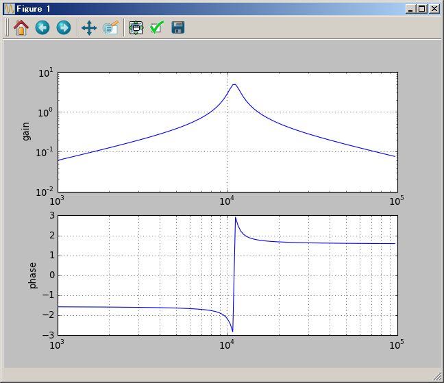
この伝達関数の極は次の PythonSf 式で求められます。
PythonSf ワンライナー
Z1,Z2,Z3,Z4,Z5 = 22kΩ`, 1kΩ`, 1/(1000pF` `s), 1/(1000pF` `s),220kΩ`; trf=Z2 Z3 Z5/(-Z1 Z2 Z3 - Z1 Z2 Z4 - Z1 Z2 Z5 - Z1 Z3 Z4 - Z2 Z3 Z4); trf.m_plDenom.roots
===============================
[-4545.45454545+68785.20886555j -4545.45454545-68785.20886555j]
uA741 オペアンプでは次のような伝達関数・Bode 線図になります。中心周波数が理想オペアンプのときより数 kHz 低くなります。
PythonSf ワンライナー
G=:uA741; Z1,Z2,Z3,Z4,Z5 = 22kΩ`, 1kΩ`, 1/(1000pF` `s), 1/(1000pF` `s),220kΩ`; trf=Z2 Z3 Z5/(-Z1 Z2 Z3 - Z1 Z2 Z4 - Z1 Z2 Z5 - Z1 Z3 Z4 - Z2 Z3 Z4 -(Z1 Z2 Z3 + Z1 Z2 Z4 + Z1 Z2 Z5 + Z1 Z3 Z4 + Z1 Z3 Z5 + Z2 Z3 Z4 + Z2 Z3 Z5)/G); trf
===============================
-2.856e+11 s
----------------------------------------
3 2
s + 7.338e+06 s + 6.214e+10 s + 2.986e+16
PythonSf ワンライナー
G=:uA741; Z1,Z2,Z3,Z4,Z5 = 22kΩ`, 1kΩ`, 1/(1000pF` `s), 1/(1000pF` `s),220kΩ`; trf=Z2 Z3 Z5/(-Z1 Z2 Z3 - Z1 Z2 Z4 - Z1 Z2 Z5 - Z1 Z3 Z4 - Z2 Z3 Z4 -(Z1 Z2 Z3 + Z1 Z2 Z4 + Z1 Z2 Z5 + Z1 Z3 Z4 + Z1 Z3 Z5 + Z2 Z3 Z4 + Z2 Z3 Z5)/G); trf.plotBode(1k` Hz`,100k` Hz`)
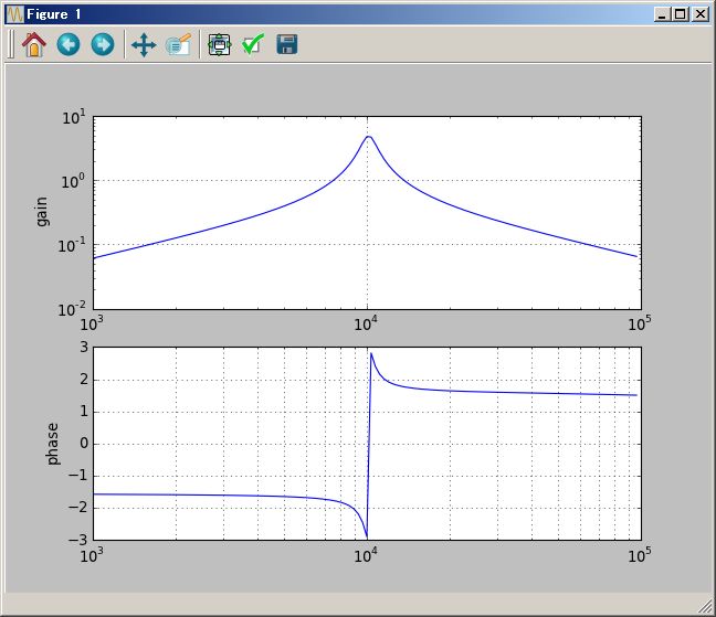
流石に複雑なトポロジーの回路で部品数も多い分、先の微分・積分回路によるバンド・パスのときより急峻な選択特性になっています。
この伝達関数の極は次の PythonSf 式で求められます。
PythonSf ワンライナー
G=:uA741; Z1,Z2,Z3,Z4,Z5 = 22kΩ`, 1kΩ`, 1/(1000pF` `s), 1/(1000pF` `s),220kΩ`; trf=Z2 Z3 Z5/(-Z1 Z2 Z3 - Z1 Z2 Z4 - Z1 Z2 Z5 - Z1 Z3 Z4 - Z2 Z3 Z4 -(Z1 Z2 Z3 + Z1 Z2 Z4 + Z1 Z2 Z5 + Z1 Z3 Z4 + Z1 Z3 Z5 + Z2 Z3 Z4 + Z2 Z3 Z5)/G); trf.m_plDenom.roots
===============================
[ -7.33006081e+06 +0.j -3.96063749e+03+63701.29330301j
-3.96063749e+03-63701.29330301j]
部品定数を変化させ根軌跡を描くことで、共振特性も検討できそうです。周波数選択特性も設計できそうです。
PythonSf 記述は数学記述に近いので、数学的な対象の説明では、自然言語による説明より PythonSf コードの方が解り易いことが多くあります。Fractal 図形について、その様子を見てみましょう。
なお、ここでは one-liner ではなく、ブロック・コードのほうが多用されます。One-liner にして再利用する意味は殆ど無いからです。ならば可読性を優先すべきだからです。
コッホ曲線を PythonSf で描きます。Wiki などにも Koch 曲線の説明があるのですが、下の 複素数を使ったコードのほうが解りやすいと思います。
PythonSf ブロック
# Koch 曲線
//@@
θ=exp(`i pi/3)
def f(lst,count=10):
if count<0:
return lst
rtn=[]
for k in range(len(lst)-1):
sg = (lst[k+1]-lst[k])/3
rtn += [lst[k], lst[k]+sg, lst[k]+sg+θ sg, lst[k]+sg 2]
rtn += [lst[-1] ]
return f(rtn, count-1)
plotTrajectory([ (x.real, x.imag) for x in f([0,1], 5)])
//@@@
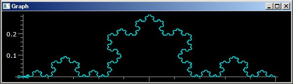
上のコードの肝は、下の二行です。
sg = (lst[k+1]-lst[k])/3
rtn += [lst[k], lst[k]+sg, lst[k]+sg+θ sg, lst[k]+sg 2]
Koch 曲線を lst に平面位置:複素数値を順番に並べることで表現します。その部分セグメント:直線:lst[k+1]-lst[k] の 1/3 の線分 sg を作ります。sg ができたら、θ sg によって左方向に 60度回転させた線分を作れます。そして [lst[k], lst[k]+sg, lst[k]+sg+θ sg, lst[k]+sg 2] によって元の線分をもう一段階細かく折り曲げた四つの繋がった線分を作ります。
下は [0,1,0.5-`i, 0] の三角形の線分から Koch 曲線を作ることで、雪の結晶のような Koch 曲線にしています。
PythonSf ブロック
# 星型の Koch 曲線
//@@
θ=exp(`i pi/3)
def f(lst,count=10):
if count<0:
return lst
rtn=[]
for k in range(len(lst)-1):
sg = (lst[k+1]-lst[k])/3
rtn += [lst[k], lst[k]+sg, lst[k]+sg+θ sg, lst[k]+sg 2]
rtn += [lst[-1] ]
return f(rtn, count-1)
plotTrajectory([ (x.real, x.imag) for x in f([0,1,0.5-`i, 0], 5)])
//@@@
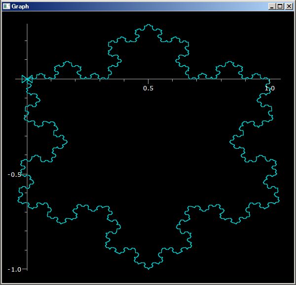
平面を埋め尽くす一次元の線として Hirbert Curve が有名です。でもWikiや WolframMathWorld などの説明を読んでも、どうやって描いていくのか簡単には理解できません。下の PythonSf ブロック・コードなら Hilbert Curve を作るアルゴリズムが良くわかると思います。いかがでしょうか?
PythonSf ブロック
//@@
N=3
# seed trajectory: matrix of position data
mt=~[(1/4,3/4),(1/4,1/4),(3/4,1/4),(3/4,3/4)]
mtL = ~[[ 0,1], # rotate pi/2 left
[-1,0]]
mtS = ~[[ 0,1], # symmetric conversion for x==y axis
[ 1,0]]
for _ in range(N):
mt=~[list((mt mtL)[::-1] +~[1,1])
+ list(mt)
+ list(mt+~[1,0])
+ list(mt mtS + ~[1,1])
]/2
plotTrajectory(mt)
//@@@
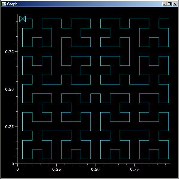
上のコードの肝は mt mtL と mt mtS の行列積です。mt は N x 2 行列であり N この平面位置ベクトルを保持しています。これに右から mtL:( pi/2 だけ回転させる) 変換と mtS:(x==y の直線に対称な位置に鏡影変換する行列を掛けることで位置ベクトルの羅列データ mt を変換しています。
標準配布の PythonSf の sfCrrntIni.py ファイルには wav ファイルを読み書きする readWv(..)/writeWv(..) 関数を書いてあります。readWv(..) 関数は wav ファイルのデータをベクトル・データに変換します。writeWv(..) 関数はベクトル・データのデータを wav ファイルに変換します。ベクトル・データであれば、PythonSf で自由に操作できます。
これを使って PythonSf one-liner による楽器音の合成や英語音声の解析を行います。
この小さな readWv(..)/wirteWv(..) カスタマイズ関数の導入だけで、PythonSf's one-liner による音声処理が可能になることを見てやってください。
pythonsf ブロック
//@@
f0=220Hz` # key 音
SR=44100Hz` # sampling rate
z_=1/`s # z^-1: z 変換記号
seed(0) # random の種
pluckedNoise=rand(SR//f0)-0.5 # 弦を引っ掛けるノイズ
F=0.996/2 (1+z_) # 減衰フィルタ 1
G=1/(1-F z_^(SR//f0)) # 減衰フィルタ 2: f0 での振動も生成する
# 伝達関数 G に pluked noise を与えたときの応答ベクトル data を作る
data=G.getDgRspns(np.r_[pluckedNoise, [0]*(SR-SR//f0)])
# 最大値を 2^15 に規格化する
data=2^15/max(abs(data))
# 規格化されたベクトル data をカレント・ディレクトリの temp.wav ファイルとして書き込む
writeWv(data, 'temp',(1, 2, SR, 32400, 'NONE', 'not compressed'))
//@@@
PythonSf ワンライナー
f0,SR,z_=220Hz`, 44100Hz`, 1/`s; seed(0);F=0.996/2 (1+z_); G=1/(1-F z_^(SR//f0)); data=G.getDgRspns(np.r_[rand(SR//f0)-0.5, [0]*(SR-SR//f0)]); data*=2^15/max(abs(data)); writeWv(data, 'temp',(1, 2, SR, 32400, 'NONE', 'not compressed'))
下のようにフィルタを追加して高周波を落としてやるとナイロン弦でのような音になります。
PythonSf ワンライナー
f0,SR,z_=220Hz`, 44100Hz`, 1/`s; seed(0); sy();y=sg.lfilter([0.1]*10,[1,1.0], rand(SR//f0)-0.5);F=0.996/4 (1+z_+z_^2+z_^3); G=1/(1-F z_^(SR//f0)); data=G.getDgRspns(np.r_[y, [0]*(SR-SR//f0)]); data=2^15/max(abs(data)) data; writeWv(data, 'temp',(1, 2, SR, 32400, 'NONE', 'not compressed'))
SciPy の signal sub package には、signal processing のための様々な関数群が用意されています。原理的には如何様なギター音でも合成できます。結構遊べます。
下のように love_rub.wav は 27545 点のデータからなり、1.728125 秒の長さの音声です。
PythonSf ワンライナーたち
readWv('love_rub').shape
==============================
(27545,)
ts(); 27645.0/(16 k` Hz`)
===============================
1.7278125*s`
WaveSurfer というソフトを使って、その波形とスペクトログラムの時間変化を下のように可視化できます。
日本人が L/R の区別をできないのは、日本語でのラ行の音に置き換えて聞いてしまうからです。love も rub も「ラブ」聞いてしまうからです。PythonSf を使って子音 L や R だけを取り出して実際に聞いてみましょう。
L の音は、love_ruv.wav ファイルで 0.358s -- 0.490s の範囲にあります。この時間幅をインデックスで表現すると、5707 -- 7011 の範囲です。下の計算で分かります。
PythonSf ワンライナーたち
# L の音の範囲のインデックスを計算する
27545 0.358s`/(1.7278125*s`)
===============================
5707.28015916
27545 0.490s`/(1.7278125*s`)
===============================
7811.64044131
7800-5700
===============================
2100
この L 子音の部分だけを抜き出して、デフォルトの _tmp.wav ファイに書き出します。ただし音声データを急激に 0 にするとプチ・ノイズになるので、最後の 200 点の音は直線状に絞って消します。したの arsq(1,200,-1/200) の部分が、それを行います。readWv(..) が「Numpy の ndarray データを返すこと」と「ndarray と list の積は要素ごとを掛け合わした ndarray でーたになること」を利用しています。
PythonSf ワンライナー
# love_rub.wav から子音 L の部分を抜き出して _tmp.wav ファイルに保存する。
vct=readWv('love_rub')[5700:7800]; writeWv(vct ( (1,)*1900+arsq(1,200,-1/200)) )
===============================
None
このようにして抜き出した子音 L の音:_tmp.wav を御自分の耳で是非とも聞いてください。日本語でのラ行の音とは異なることが分かると思います。この子音 L の部分だけ(母音とは独立させて)聞き取れるようになると L/R の誤認識を改善できます。
でもまだ この子音:L には余分なノイズに近い音が混じっています。私が L の音だと思っているのとは少し違いがあります。その L の音を抜き出すため、フーリエ変換を使います。
PythonSf ワンライナー
# 子音 L のフーリエ変換
vc=readWv('_tmp'); plotGr( abs( fftshift( fft(vc) ) ) )
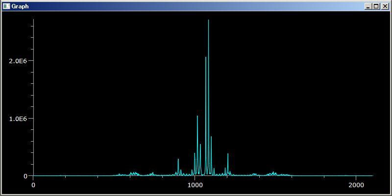
上のグラフでフーリエ変換の絶対値のグラフは左右対称です。画面で左右対称になっていないのは、2100 点のデータをコンピュータ画面上で表示するときに歯抜けが発生するからです。歯抜けが左右対称には起きないためです。1000 点のデータ:±4kHz 弱の領域に限ると、下のように左右対称になります。
PythonSf ワンライナー
# 子音 L のフーリエ変換結果を中心部分 1000 点に限定してグラフ化する
vc=readWv('_tmp'); plotGr( abs( fftshift( fft(vc) ) )[2100/2-550: 2100/2+550] )
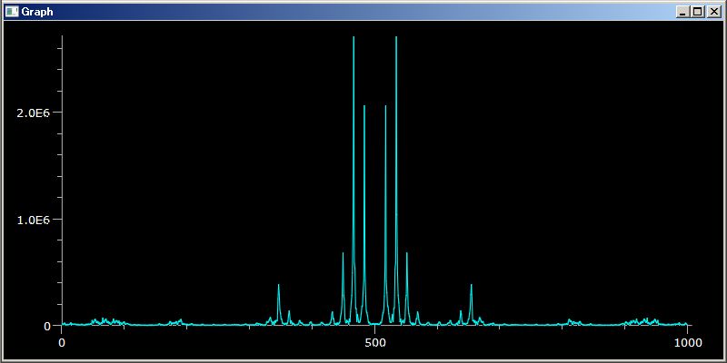
PythonSf ワンライナーたち
# 16kHz サンプリングの fft データから 220 点のデータを取り出したときの周波数
16k` Hz` 220/2100
===============================
1676.19047619
# 子音 L の音を±1.6kHz に限定した _tmp.wav ファイルを作る
vc=readWv('_tmp'); v=fft(vc); v[220:-220]=0; writeWv( ifft(v).real )
上のようにして作った _tmp.wav ファイルの音を自分の耳で聞いて見てください。love の音から、この部分の音に集中して聞き取るようにすることで love の英語の l が、日本語のラブとは違った音として聞き取れるようになってきます。